The role of wave–wave interactions in sudden stratospheric warming formation

Lindgren, Erik A.; Sheshadri, Aditi

doi:https://doi.org/10.5194/wcd-1-93-2020

Articles | Volume 1, issue 1

https://doi.org/10.5194/wcd-1-93-2020

Articles | Volume 1, issue 1

Research article

10 Mar 2020

Research article |

| 10 Mar 2020

The role of wave–wave interactions in sudden stratospheric warming formation

Erik A. Lindgren and Aditi Sheshadri

Abstract

The effects of wave–wave interactions on sudden stratospheric warming formation are investigated using an idealized atmospheric general circulation model, in which tropospheric heating perturbations of zonal wave numbers 1 and 2 are used to produce planetary-scale wave activity. Zonal wave–wave interactions are removed at different vertical extents of the atmosphere in order to examine the sensitivity of stratospheric circulation to local changes in wave–wave interactions. We show that the effects of wave–wave interactions on sudden warming formation, including sudden warming frequencies, are strongly dependent on the wave number of the tropospheric forcing and the vertical levels where wave–wave interactions are removed. Significant changes in sudden warming frequencies are evident when wave–wave interactions are removed even when the lower-stratospheric wave forcing does not change, highlighting the fact that the upper stratosphere is not a passive recipient of wave forcing from below. We find that while wave–wave interactions are required in the troposphere and lower stratosphere to produce displacements when wave number 2 heating is used, both splits and displacements can be produced without wave–wave interactions in the troposphere and lower stratosphere when the model is forced by wave number 1 heating. We suggest that the relative strengths of wave number 1 and 2 vertical wave flux entering the stratosphere largely determine the split and displacement ratios when wave number 2 forcing is used but not wave number 1.

Download & links

Article (PDF, 10174 KB)

Supplement (698 KB)

Download & links

Article (10174 KB)
Supplement (698 KB)
BibTeX
EndNote

How to cite

How to cite.

Dates

Received: 13 Sep 2019 – Discussion started: 24 Sep 2019 – Revised: 29 Jan 2020 – Accepted: 19 Feb 2020 – Published: 10 Mar 2020

1 Introduction

Sudden stratospheric warmings (SSWs) are dynamical events that can occur during hemispheric winter and which result in a collapse of the stratospheric polar vortex. During SSWs the temperature of the middle and upper polar stratosphere increases by over 30 K over a period of a few days (Butler et al., 2015), and the strongest SSWs, often called major SSWs, are usually defined by a reversal of the zonal-mean westerlies at 60^∘ and 10 hPa (Charlton and Polvani, 2007). Accurate simulations of SSWs in models are crucial for capturing the variability in surface climate in midlatitudes, since the effects of SSWs can migrate down to the troposphere and can impact surface weather up to 2 months after onset (e.g., Baldwin and Dunkerton, 2001). During SSWs the stratospheric polar vortex is either displaced from the pole as a single entity or split into two daughter vortices. These two types of SSWs are known as displacements and splits, and they are dominated by zonal wave number 1 and 2 disturbances, respectively. It has been suggested that splits and displacements are dynamically distinct (Charlton and Polvani, 2007; Matthewman et al., 2009), and some studies claim that they may have different surface impacts (e.g., Mitchell et al., 2013; Seviour et al., 2013; Lindgren et al., 2018), while others have found that differences in surface impacts are not consistent for different split and displacement classifications and that large numbers of events are required to distinguish any differences (Maycock and Hitchcock, 2015). Major SSWs occur about every other year in the Northern Hemisphere and are roughly equally distributed between splits and displacements (Charlton and Polvani, 2007; Lindgren et al., 2018, and others). Only one major SSW has been observed in the Southern Hemisphere (e.g., Allen et al., 2003).

Despite their importance for Northern Hemispheric climate variability, the dynamics behind SSW generation remain poorly understood. SSWs can occur when waves propagate from the troposphere to the stratosphere, where they break and deposit momentum (e.g., Matsuno, 1971), and from this perspective SSWs can be considered wave–mean flow interactions. It has long been known that SSW-like zonal-mean wind variations can occur in model setups as simple as one-dimensional β-plane models (e.g., Holton and Mass, 1976; Yoden, 1990). SSW generation in general circulation models (GCMs) and the observed atmosphere, however, is likely much more complicated. Although anomalously strong tropospheric wave forcing can produce SSWs, SSW-like events have been found to occur in idealized GCMs with suppressed tropospheric variability (Scott and Polvani, 2004, 2006), and recent research has shown that only about a third of SSWs and SSW-like events are associated with anomalous tropospheric wave forcing. This has been shown in reanalysis data (Birner and Albers, 2017; de la Cámara et al., 2019), chemistry–climate models (de la Cámara et al., 2019; White et al., 2019), and one idealized GCM (Lindgren et al., 2018). Birner and Albers (2017) argued that the dynamical processes responsible for most SSWs occur just above the tropopause, even though the wave forcing responsible for the events originates near the surface. The importance of stratospheric processes in SSW dynamics was also emphasized by Hitchcock and Haynes (2016), who found that the evolution of the stratospheric mean state during SSWs is crucial in determining the wave flux during the warming. Given the complexity of SSW generation it is not possible to predict how frequently, or even if, SSWs will occur in a given model setup a priori, and idealized GCMs are therefore often extensively tuned to produce realistic SSW frequencies (e.g., Gerber and Polvani, 2009; Sheshadri et al., 2015; Lindgren et al., 2018).

Exactly which dynamical processes are responsible for vortex splits and displacements is also unclear. Since displacements and splits are zonal wave number 1 and 2 disturbances, respectively, one could expect that the zonal wave number of the wave flux propagating from the troposphere will determine the type of SSW produced. Large-scale topography of a single, zonal wave number has often been used to produce Northern Hemisphere winter-like stratospheric variability in idealized GCMs, and in such cases the wave number of the topography does indeed strongly influence the type of SSW produced, with wave number 1 (wave 1) topography favoring displacements (Martineau et al., 2018) and wave number 2 (wave 2) topography producing mostly or only splits (Gerber and Polvani, 2009; Sheshadri et al., 2015; Martineau et al., 2018; Lindgren et al., 2018). Recently, however, Lindgren et al. (2018) showed that splits and displacements occur in comparable amounts when an idealized GCM is forced with wave 1 or wave 2 tropospheric heating perturbations. Since the tropospheric forcings are of pure wave 1 or 2 format these results indicate that some wave–wave interaction could take place somewhere between the waves being forced in the troposphere and the waves breaking in the stratosphere.

Idealized models are useful tools when investigating specific dynamical processes, and simple models have frequently been used in previous studies of SSW dynamics. After one-dimensional β-plane models (e.g., Holton and Mass, 1976; Yoden, 1990) the next step in the model hierarchy includes the effects of wave–wave interactions (WWIs), and research about the role of WWIs in stratospheric dynamics dates back to the 1980s. Lordi et al. (1980) applied wave 1 and 2 geopotential height forcings at the lower boundary of a primitive-equation spectral model of the stratosphere to simulate SSWs. They used spectral truncation to remove interactions between wave numbers and only allowed the wave number of the forcing to interact with the mean flow. They concluded that nonlinear interactions are important for the evolution of the mean flow and temperature fields in the middle and upper stratosphere, especially when wave 1 forcing was used. Austin and Palmer (1984) used a primitive-equation model of the stratosphere and mesosphere to investigate the role of nonlinear effects in setting up the monthly mean wave amplitudes in the stratosphere during December 1980 and concluded that WWIs cannot be ignored for accurate simulations of the middle atmosphere.

O'Neill and Pope (1988) carried out an extensive study of linear and nonlinear disturbances in the stratosphere resulting from tropospheric perturbations, with the same primitive-equation model that Austin and Palmer (1984) used. They found that linear theories of wave propagation and wave–mean flow interaction were useful when the imposed lower boundary forcing was weak but that the stratospheric flow was highly nonlinear in the latter stages of simulations with strong forcing. Their results suggested that major stratospheric warmings evolve from highly asymmetric states through complicated nonlinear interactions rather than simple wave–mean flow interactions.

Robinson (1988) simulated a minor wave 1 stratospheric warming in a primitive-equation model, while running the model in a fully nonlinear mode as well as in a quasi-linear mode, with waves of only one wave number and the zonal flow. The model runs were 60 d long following the spin-up period. He found that irreversible modifications of the potential vorticity field were stronger and more localized when WWIs were allowed and that the differences between the nonlinear and quasi-linear model runs come from modifications of the interactions between wave 1 and the zonal flow by shorter waves. The interactions between shorter waves and the mean flow were found to be of much less importance when accounting for the differences between the experiments.

There is also observational evidence to suggest that WWIs are largely responsible for modulating the relative strengths of wave 1 and wave 2 disturbances in the stratosphere. Smith et al. (1983) used satellite data to investigate the importance of wave–mean flow interactions versus WWIs in the Northern Hemisphere during the 1978–1979 winter and found that vacillations between wave 1 and wave 2 in the geopotential height field could be largely attributed to WWIs in the stratosphere rather than forcing from the tropopause region.

The authors mentioned above have shown that WWIs play an important role in stratospheric dynamics in general and SSW dynamics in particular, but many questions regarding the role of WWIs in SSW dynamics remain unanswered. One major restriction of the previous studies is that spectral truncation was used to eliminate WWIs while keeping only the interactions between a single wave number and the mean flow (Lordi et al., 1980; Robinson, 1988). The climatological wave flux in the observed stratosphere contains both wave 1 and wave 2 components (e.g., Birner and Albers, 2017), both of which can interact with the mean flow. Given that displacements and splits are wave 1 and wave 2 disturbances, respectively, removal of either of the major stratospheric wave numbers along with WWIs will enable only one type of SSW to form even though SSWs in the observed atmosphere are roughly equally distributed between splits and displacements (Charlton and Polvani, 2007; Lindgren et al., 2018, and others). Other limitations of previous work include the short temporal extents and coarse resolutions of the model runs, due to the limited computing resources of the 1980s. It is known that WWIs are important both for SSW generation (O'Neill and Pope, 1988) and the evolution of the stratospheric mean state during SSWs (Hitchcock and Haynes, 2016), but the effect that WWIs have on SSW frequencies has not been investigated, and it is not clear a priori whether WWIs act to enhance or diminish SSW generation.

Furthermore, previous work has removed WWIs throughout the vertical extent of the models even though the dynamics of the troposphere, tropopause region and stratosphere are very different. Birner and Albers (2017) emphasized the importance of dynamics in the 300–200 hPa region (just above the tropopause) for SSW formation. Polvani and Waugh (2004) found that anomalous wave fluxes at 100 hPa and further down in the troposphere precede SSWs and deduced that the origin of SSWs can be found in the troposphere (although they acknowledged the fact that the stratosphere may play a role in modulating the events). These results indicate that dynamical processes in the troposphere and lower stratosphere are crucial in SSW formation, which raises the question as to whether or not the role of WWIs in SSW dynamics varies accordingly. The recent results of Lindgren et al. (2018) show that both splits and displacements can form with a tropospheric forcing of a single wave number, indicating that WWIs could act to transfer energy from the wave number of the forcing to the other major stratospheric wave number somewhere between the troposphere and the stratosphere. In order to understand the importance of WWIs for SSW generation as well as split and displacement distributions at different vertical levels in the atmosphere, a different method of removing WWIs must be used.

More recently, the effects of WWIs on atmospheric dynamics have been investigated in idealized models by calculating the advection of eddy fluctuations by eddy winds and replacing them with their zonal-mean values. Unlike the spectral truncation mentioned in the papers above, this method allows climatological wave flux of all wave numbers to interact with the mean flow, and it retains much of the zonal-mean climatology of (nonlinear) control runs. The method has been successfully used to investigate tropospheric dynamics by several authors: O'Gorman and Schneider (2007) removed WWIs in an idealized GCM and found that the atmospheric kinetic energy spectrum retained its wave number dependence when WWIs were removed even though this dependence was previously thought to be determined by WWIs. Chemke and Kaspi (2016) showed that WWIs in an idealized GCM actually decrease the number of eddy-driven jets in the atmosphere by narrowing the latitudinal region where zonal jets can appear. This method has also proven useful when applied to theories of jet dynamics in β-plane models (e.g., Srinivasan and Young, 2012; Tobias and Marston, 2013; Constantinou et al., 2014).

In this paper we investigate the role of WWIs in SSW formation by removing the effects of zonal WWIs in an idealized GCM, using the method of O'Gorman and Schneider (2007). We use the model output produced with heating wave 1 (H1) and wave 2 (H2) tropospheric forcing from Lindgren et al. (2018), both of which produce splits and displacements in comparable amounts even though the forcings are of a single wave number. This makes the model setups ideal for studying the role of WWIs in SSW generation in general and split and displacement formation in particular. We perform model runs under three additional settings for each forcing: one without WWIs anywhere, one without WWIs in the troposphere and lower stratosphere, and one without WWIs in the middle and upper stratosphere. The latter two, hereafter referred to as the mixed runs, allow us to investigate the effects of removing WWIs below (above) the vertical levels that Polvani and Waugh (2004) and Birner and Albers (2017) highlighted as crucial for SSW generation while still allowing WWIs above (below). By comparing the results of the mixed runs to the fully nonlinear control runs and the model runs without WWIs anywhere, we can investigate the importance of WWIs in the middle and upper stratosphere when the climatology (and hence mean wave forcing) in the troposphere and lower stratosphere remains unchanged. We use the model runs to answer three questions related to WWIs and SSW formation that have not been investigated before:

To what extent do WWIs affect SSW frequencies?
To what extent are the numbers of splits and displacements, and their ratios, affected by WWIs?
How do WWIs affect SSWs frequencies and split and displacement ratios when the lower-stratospheric wave forcing does not change?

We find that the effects of WWIs on SSWs are strongly dependent on the wave number of the tropospheric forcing. We show that the absence of WWIs can significantly alter SSW frequencies and that whether WWIs increase or decrease SSW frequencies depends on the tropospheric forcing that is used and the vertical levels where WWIs are removed. Significant changes in SSW frequencies between model runs with and without WWIs in the middle and upper stratosphere are obtained even though the lower-stratospheric wave forcings of the model runs do not change, highlighting the fact that the stratosphere is not a passive recipient of lower-stratospheric wave forcing. We further find that while WWIs are required in the troposphere and lower stratosphere to produce displacements when wave 2 forcing is used, both splits and displacements can be produced without WWIs in the troposphere and lower stratosphere when the model is forced by wave 1 heating.

Section 2 describes the method used to remove the effects of WWIs and the way it was implemented in the model runs. Section 3 describes changes in climatology caused by removal of WWIs. Section 4 compares the SSW frequencies, split and displacement ratios, and polar vortex strength variabilities in the eight different model runs. A discussion of the results and conclusions can be found in Sect. 5.

2 Removal of wave–wave interactions

Following O'Gorman and Schneider (2007), we calculated the tendency due to zonal WWIs (the wave–wave tendency), subtracted it from the total tendency of horizontal wind and temperature, and added the zonal-mean value of the wave–wave tendency (the mean tendency) to the total tendency equation. This method removes interactions between zonal waves. This substitution was described by O'Gorman and Schneider (2007) by using the equation for temperature tendency as an example. In the control run the evolution is

\begin{matrix} (1) & \begin{aligned} \frac{\partial T}{\partial t} & = - v \frac{\partial T}{\partial y} + \dots \\ = - \overline{v} \frac{\partial \overline{T}}{\partial y} - \overline{v} \frac{\partial T^{'}}{\partial y} - v^{'} \frac{\partial \overline{T}}{\partial y} - v^{'} \frac{\partial T^{'}}{\partial y} + \dots, \end{aligned} \end{matrix}

where overbars denote zonal means while primes show deviations from the zonal mean (eddies, or waves). Only the terms related to meridional advection of temperature were written out. The last term in Eq. (1) describes the advection of temperature eddies due to meridional wind eddies. In the model runs where WWIs are not allowed Eq. (1) becomes

\begin{matrix} (2) & \begin{aligned} \frac{\partial T}{\partial t} & = - v \frac{\partial T}{\partial y} + \dots \\ = - \overline{v} \frac{\partial \overline{T}}{\partial y} - \overline{v} \frac{\partial T^{'}}{\partial y} - v^{'} \frac{\partial \overline{T}}{\partial y} - \overline{v^{'} \frac{\partial T^{'}}{\partial y}} + \dots, \end{aligned} \end{matrix}

where the contribution due to WWIs was replaced by its zonal-mean value. It should be noted that this method only removes interactions between zonal waves and that meridional WWIs are still allowed. However, it is zonal flow over the continents, oceans and large-scale topography that produces the planetary-scale waves which propagate into the stratosphere, and the WWIs important for stratospheric dynamics therefore occur between zonal waves. Unless otherwise noted, WWIs hereafter refer to zonal WWIs.

Two model runs from Lindgren et al. (2018) are used in this paper. The GCM is a dry, hydrostatic, global primitive-equation model with T42 resolution in the horizontal and 40 vertical σ levels, where $σ = p / p_{s}$ . The model setup is based on that of Polvani and Kushner (2002). There are no convection or radiation schemes in the model, and temperature is relaxed towards a zonally symmetric temperature profile through Newtonian relaxation. The temperature profile is symmetric about the Equator in the troposphere and identical to that of Held and Suarez (1994) but set to perpetual Northern Hemisphere midwinter conditions in the stratosphere. The transition between tropospheric and stratospheric equilibrium temperature profiles occurs at 200 hPa. Tropospheric diabatic heating perturbations are used to produce Northern Hemisphere winter-like stratospheric variability. The reader is referred to Lindgren et al. (2018) for more information about the model and heating perturbations. In addition to the H1 and H2 runs from Lindgren et al. (2018) another three runs were performed for each forcing wave number, where each of the three additional runs removed WWIs in different parts of the atmosphere. All model setups were run under Northern Hemisphere winter conditions for 31 100 d, and the last 30 000 d were used for the analysis. The vertical structures of where WWIs are permitted and removed can be found in Figs. 1 and 2.

http://www.weather-clim-dynam.net/1/93/2020/wcd-1-93-2020-f01

Figure 1Vertical structure of the four runs used for each wave number (1 or 2). See text for details.

Download

http://www.weather-clim-dynam.net/1/93/2020/wcd-1-93-2020-f02

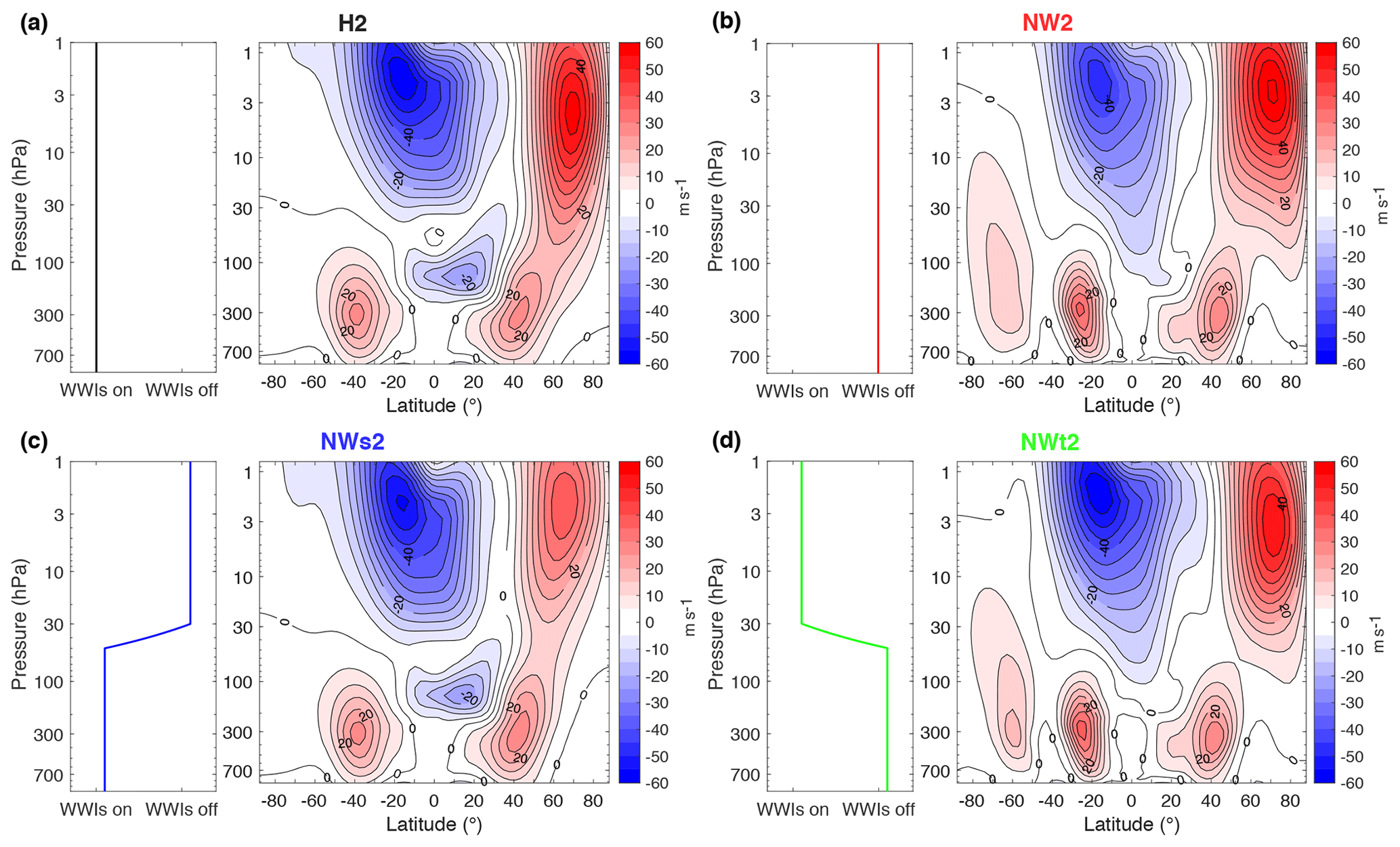
Figure 2Zonal-mean zonal winds for H2 (a), NW2 (b), NWs2 (c) and NWt2 (d), with panels showing the pressure levels where WWIs are allowed. The contour interval is 5 ms⁻¹.

Download

In the control runs (H1 and H2; black line in Figs. 1 and 2) WWIs are allowed everywhere. In the no-WWIs-anywhere runs (NW1 or NW2 depending on the wave number of the forcing; red line) the effects of WWIs were removed at each pressure level. In the mixed runs the model is set up to switch between allowing and not allowing WWIs linearly with pressure. The transition occurs between 50 and 30 hPa. In the case of the runs with no WWIs allowed in the troposphere and lower stratosphere (hereafter shortened as NWt1 or NWt2; green line) the following substitution is made:

\begin{matrix} (3) & \frac{\partial T}{\partial t} = \{\begin{cases} \frac{\partial T}{\partial t} - \overline{v^{'} \frac{\partial T^{'}}{\partial y}} + v^{'} \frac{\partial T^{'}}{\partial y}, p > p_{1}, \\ \frac{\partial T}{\partial t} + (1 - \frac{p_{1} - p}{p_{1} - p_{2}}) \cdot (- \overline{v^{'} \frac{\partial T^{'}}{\partial y}} + v^{'} \frac{\partial T^{'}}{\partial y}), \\ p_{2} \leq p \leq p_{1}, \\ \frac{\partial T}{\partial t}, p < p_{2} . \end{cases} \end{matrix}

In the above equation the temperature tendency from Eqs. (1) and (2) was used as an example. p₁=50 hPa and p₂=30 hPa. Similarly, when WWIs are not allowed in the upper stratosphere (hereafter shortened as NWs1 or NWs2; blue line) the equation describing the substitution is

\begin{matrix} (4) & \frac{\partial T}{\partial t} = \{\begin{cases} \frac{\partial T}{\partial t}, p > p_{1}, \\ \frac{\partial T}{\partial t} + \frac{p_{1} - p}{p_{1} - p_{2}} \cdot (- \overline{v^{'} \frac{\partial T^{'}}{\partial y}} + v^{'} \frac{\partial T^{'}}{\partial y}), \\ p_{2} \leq p \leq p_{1}, \\ \frac{\partial T}{\partial t} - \overline{v^{'} \frac{\partial T^{'}}{\partial y}} + v^{'} \frac{\partial T^{'}}{\partial y}, p < p_{2} . \end{cases} \end{matrix}

The mixed runs enable an investigation of the effects of WWIs in different regions of the atmosphere. Although it may seem an obvious choice to put the transition region around the tropopause this alters the climatologies of the mixed runs significantly compared to the control runs, something that is likely caused by substantial changes in the strong climatological wave convergence just above the tropopause (see Figs. 3 and 4). Furthermore, the heating perturbation from Lindgren et al. (2018) reaches up to 200 hPa, which puts a small part of the perturbation in the lower stratosphere. Therefore, the 50 and 30 hPa levels were chosen as start and end points of the transition region. This choice has three strong advantages over the tropopause region: first, it is an unusually calm region of the atmosphere in terms of wave activity, and changes in wave interactions do not affect the climatology as strongly. Second, it is located well above the extent of the heating perturbation, so no part of the wave forcing crosses the transition region. Third, the pressure levels where lower-stratospheric wave forcing has been highlighted as important for SSWs range from 300–200 hPa (Birner and Albers, 2017) to 100 hPa (Polvani and Waugh, 2004). The choice of a transition region between 50 and 30 hPa as opposed to the tropopause means that we can keep what is thought to be the most important wave forcing identical between model runs that allow (remove) WWIs everywhere and turn WWIs off (on) in the middle and upper stratosphere.

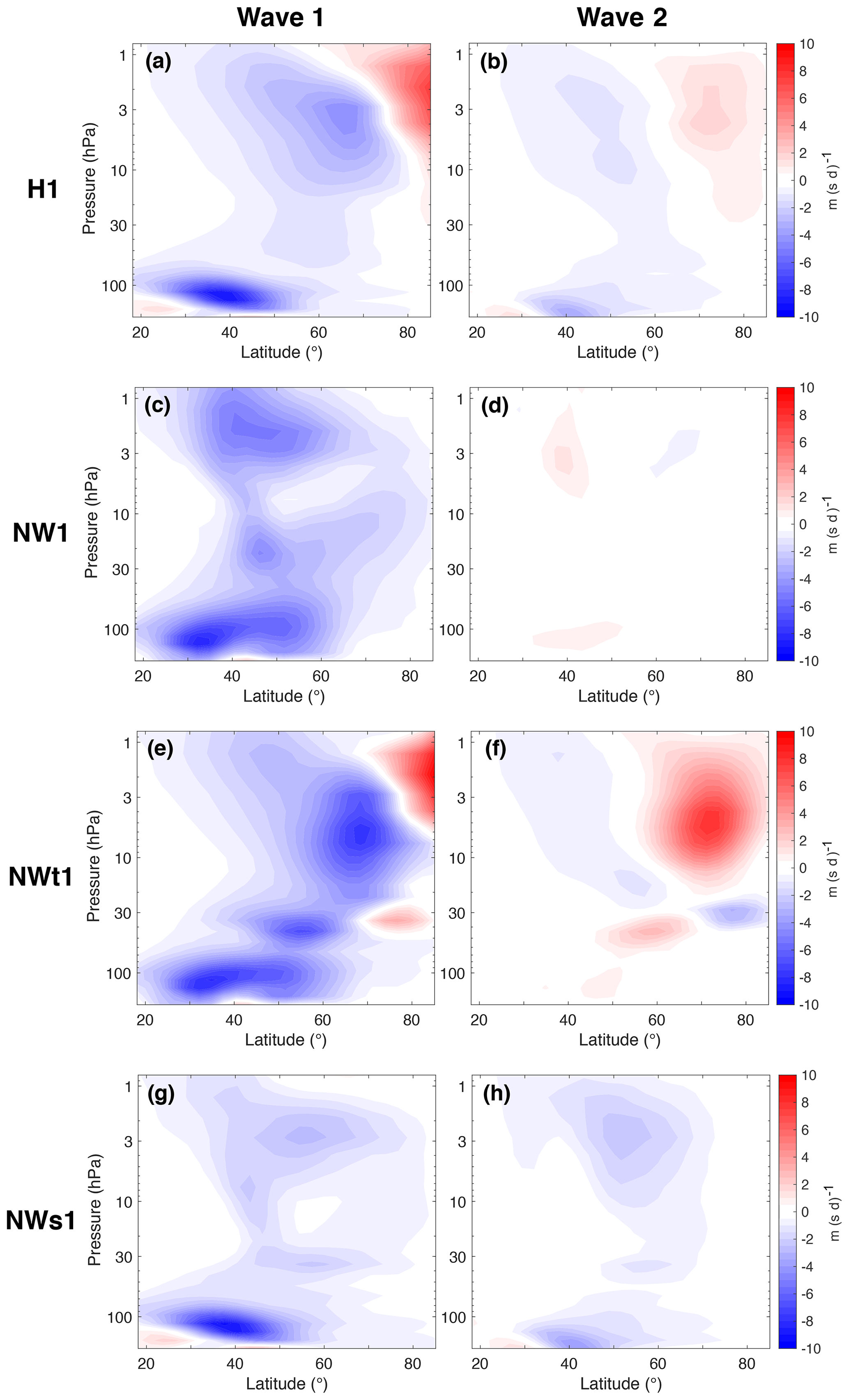
http://www.weather-clim-dynam.net/1/93/2020/wcd-1-93-2020-f03

Figure 3Divergence of EP flux for H1 (a, b), NW1 (c, d), NWt1 (e, f) and NWs1 (g, h). (a, c, e, g) Wave 1 components. (b, d, f, h) Wave 2 components. The contour interval is 0.5 m (s d)⁻¹.

Download

3 Climatology in the absence of WWIs

Figure 2 shows the climatological zonal-mean zonal wind for the four model runs with wave 2 heating along with panels indicating the pressure levels where WWIs are allowed. Zonal-mean zonal winds for model runs with wave 1 heating can be found in the Supplement (Supplement Fig. S1). A comparison of H2 (Fig. 2a) to NW2 (Fig. 2b) shows that the model retains much of the climatological zonal-mean zonal wind structure even in the absence of WWIs, although with some notable exceptions. For one, the polar night jet is much more separated from the tropospheric jet when WWIs are not allowed in the troposphere and lower stratosphere (Fig. 2b and d). The jet strength, however, is largely unaffected in NW2. This is not the case in all model runs, especially NWs2 (Fig. 2c) compared to the other model runs with wave 2 heating. The area where the zonal-mean zonal wind approaches zero meters per second found in the equatorial lower stratosphere in the control runs is not reproduced when WWIs are not allowed in the troposphere and lower stratosphere (Fig. 2b and d), indicating that WWIs play an important role in this area. Furthermore, there are two tropospheric jets in the Southern Hemisphere in these runs. O'Gorman and Schneider (2007) and Chemke and Kaspi (2016) also obtained additional tropospheric jets in their models when removing WWIs, and Chemke and Kaspi (2016) showed that WWIs decrease the number of eddy-driven jets in the atmosphere.

Comparisons between the mixed runs and H2 or NW2 show that changes in the middle and upper stratosphere have very little influence on the climatology of the troposphere and lower stratosphere. When WWIs are allowed in the troposphere and lower stratosphere only (NWs2; Fig. 2c) the zonal-mean zonal winds at vertical levels below 50 hPa are very similar to those of the control run (H2; Fig. 2a). Similarly, when WWIs are not allowed in the troposphere and lower stratosphere (NWt2; Fig. 2d) the climatology at vertical levels below 50 hPa is very similar to that of the model run where WWIs are not allowed anywhere (NW2; Fig. 2b). The same is true when wave 1 heating is used; see Fig. S1.

To investigate the changes in wave activity caused by removing WWIs we calculated the climatological wave 1 and wave 2 components of vertical Eliassen–Palm (EP) flux (F_p) and divergence of EP flux for the eight model runs. The calculations were based on Edmon et al. (1980) and are identical to those found in Lindgren et al. (2018). Although waves of higher wave numbers also interact with each other and the mean flow (especially in the troposphere), we focus our attention on wave numbers 1 and 2 below since only large-scale waves can propagate into the stratosphere (e.g., Charney and Drazin, 1961) and since these are the wave numbers of the tropospheric forcings. Figures 3 through 6 show the wave 1 and wave 2 components of the two quantities. The most important result of the EP flux figures is that, just like the zonal-mean zonal wind in Fig. 2, the divergence of EP flux and F_p at vertical levels below 50 hPa depend on whether or not WWIs are allowed at these levels: NW1 and NW2 look very similar to NWt1 and NWt2, while H1 and H2 look like NWs1 and NWs2 in this region. This indicates that changing the conditions for WWIs above 50 hPa does not affect the climatological wave forcing from lower levels, and it will enable us to shed light on the importance of the middle and upper stratosphere for SSW generation compared to the 300–200 hPa (Birner and Albers, 2017) and 100 hPa (Polvani and Waugh, 2004) levels highlighted by previous authors.

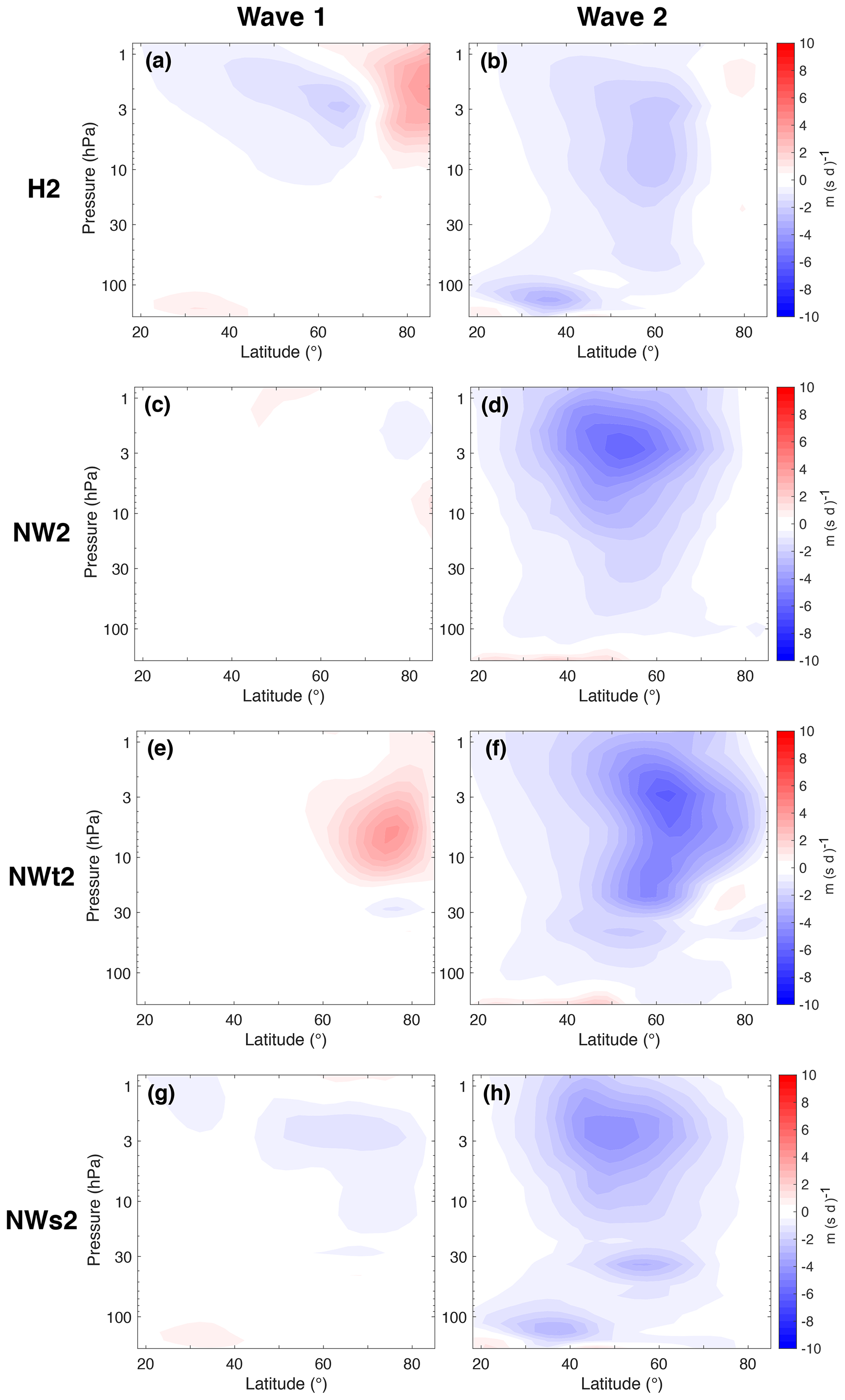
http://www.weather-clim-dynam.net/1/93/2020/wcd-1-93-2020-f04

Figure 4Divergence of EP flux for H2 (a, b), NW2 (c, d), NWt2 (e, f) and NWs2 (g, h). (a, c, e, g) Wave 1 components. (b, d, f, h) Wave 2 components. The contour interval is 0.5 m (s d)⁻¹.

Download

There are substantial wave 1 and wave 2 EP flux divergence components in the stratosphere of both H1 and H2 (Fig. 3a and b and Fig. 4a and b), which shows that there is a large amount of both wave 1 and wave 2 activity in the two control runs. This results in large numbers of both splits and displacements in both runs (Lindgren et al., 2018). In contrast, removal of WWIs everywhere results in an EP flux divergence completely dominated by the wave number of the forcing, with practically only wave 1 and no wave 2 EP flux convergence in NW1 (Fig. 3c and d), while the opposite is true for NW2 (Fig. 4c and d). This result is not surprising: removal of WWIs means that waves can only interact with the mean flow, which excludes the possibilities of energy transfer between wave numbers. In contrast, there are areas of EP flux divergence of a wave number different from that of the tropospheric forcing just above the transition region in NWt1 and NWt2 (Figs. 3f and 4e), and areas of EP flux convergence in the same region in the wave number of the forcing (Fig. 3e and 4f). This suggests that once WWIs are allowed some of the wave activity is transferred from the wave number of the forcing to the other of the two major stratospheric wave numbers. Another aspect worth noting is that the areas of strongest F_p and EP flux convergence occur further poleward when WWIs are allowed in the stratosphere compared to when they are not. This does not seem to be a result of changing zonal wind climatology and hence a shift in the structure of the wave guide, since the latitudinal polar night jet shifts between the model configurations are modest (Figs. 2 and S1). Robinson (1988) found that removal of all waves but wave 1 resulted in a more equatorward wave flux compared to his nonlinear model run. He deduced that this difference came from the removal of interactions between wave 1 and shorter waves and that interactions between shorter waves and the mean flow had a comparably small effect on the wave flux. Our results confirm the conclusion of Robinson (1988), since our experiments allow interactions between all waves and the mean flow, and the equatorward shift persists.

4 Impacts on SSWs and polar vortex strength

Table 1 shows the SSW frequencies, time mean and variability in zonal-mean zonal wind at 10 hPa and 60^∘ N, and split and displacement ratios for the eight runs. A SSW is defined here as a reversal of the zonal-mean westerlies at 60^∘ N and 10 hPa with at least 20 d of consecutive westerlies between events (Charlton and Polvani, 2007). The SSW frequency is one way to characterize the variability in the stratospheric polar vortex, but it is a binary definition and not wholly representative of stratospheric variability. The time mean and variability in zonal-mean zonal wind at the same pressure level and latitude therefore provide further metrics for how changes in WWIs affect the polar vortex strength. The wave amplitude classification (WAC) introduced by Lindgren et al. (2018) was used to classify the SSWs as splits or displacements. We use a Monte Carlo approach to assess the statistical significance of differences in SSW frequencies and split and displacement ratios at a 95 % confidence level; the method is described in detail in the Supplement.

Table 1SSW frequencies, time mean and variability in $\overline{u}$ at 10 hPa and 60^∘ N, and classifications for the model runs. Split and displacement numbers are obtained with a wave amplitude classification; numbers in square brackets indicate that the SSWs do not look like typical splits or displacements.

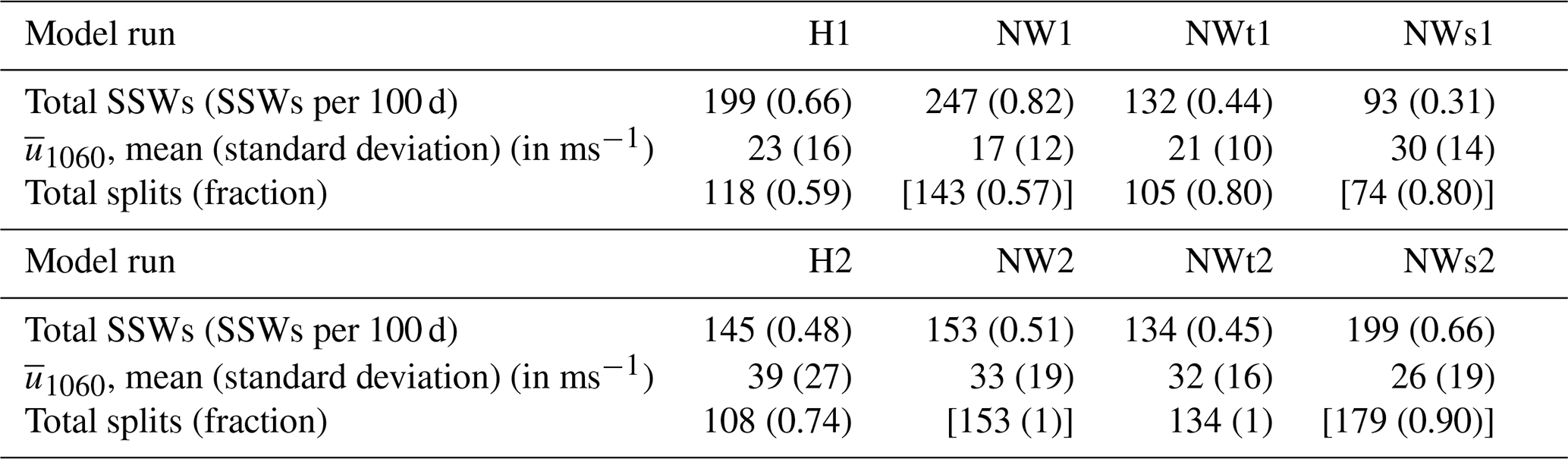
Download Print Version | Download XLSX

Removal of WWIs affects SSW frequencies significantly when the model is forced by wave 1 heating. The SSW frequency in H1 is 0.66 SSWs per 100 d, but in NW1 the frequency is increased to 0.82 (a 24 % increase). The frequencies are lower in the mixed runs: 0.44 in NWt1 and 0.31 in NWs1 (decreases of 34 % and 53 % compared to the control run, respectively). The differences between these model runs are all statistically significant. It is reasonable that the SSW frequencies in the wave 1 runs should be affected by removal of WWIs, since WWIs affect the climatological wave forcing quite strongly with this heating perturbation. Figure 5 shows that there are strong tropospheric wave 1 and wave 2 components of F_p in H1 but that the wave 2 component disappears when WWIs are not allowed in the troposphere. However, the results from the mixed runs are more surprising: removal of WWIs in the middle and upper stratosphere only (NWs1) decreases the SSW frequency by over 50 % compared to the control run. Similarly, allowing WWIs in the middle and upper stratosphere only (NWt1) decreases the SSW frequency by 45 % compared to NW1. As was mentioned in the previous section, the tropospheric and lower-stratospheric wave forcing depends on whether or not WWIs are allowed at these levels and not on the conditions in the middle and upper stratosphere. The fact that the wave forcings and climatologies below 50 hPa in H1 and NWs1 as well as NW1 and NWt1 are practically identical while their SSW frequencies are very different shows that WWIs in the stratosphere play a major role in SSW generation. Supporting the conclusions of Hitchcock and Haynes (2016), it also highlights the fact that the upper stratosphere is not a passive recipient of wave forcing from below, even though the importance of tropospheric and lower-stratospheric wave forcing for SSW generation has often been emphasized (Polvani and Waugh, 2004; Birner and Albers, 2017). Like O'Neill and Pope (1988), we find that SSWs cannot simply be considered forced by wave–mean flow interactions from a lower boundary. However, there is no clear answer to how WWIs in the middle and upper stratosphere influence SSW frequencies with wave 1 forcing: a comparison between H1 and NWs1 suggests that WWIs are necessary in the middle and upper stratosphere to get high SSW frequencies, while the results for NW1 and NWt1 indicate that allowing WWIs in the middle and upper stratosphere decreases the SSW frequency.

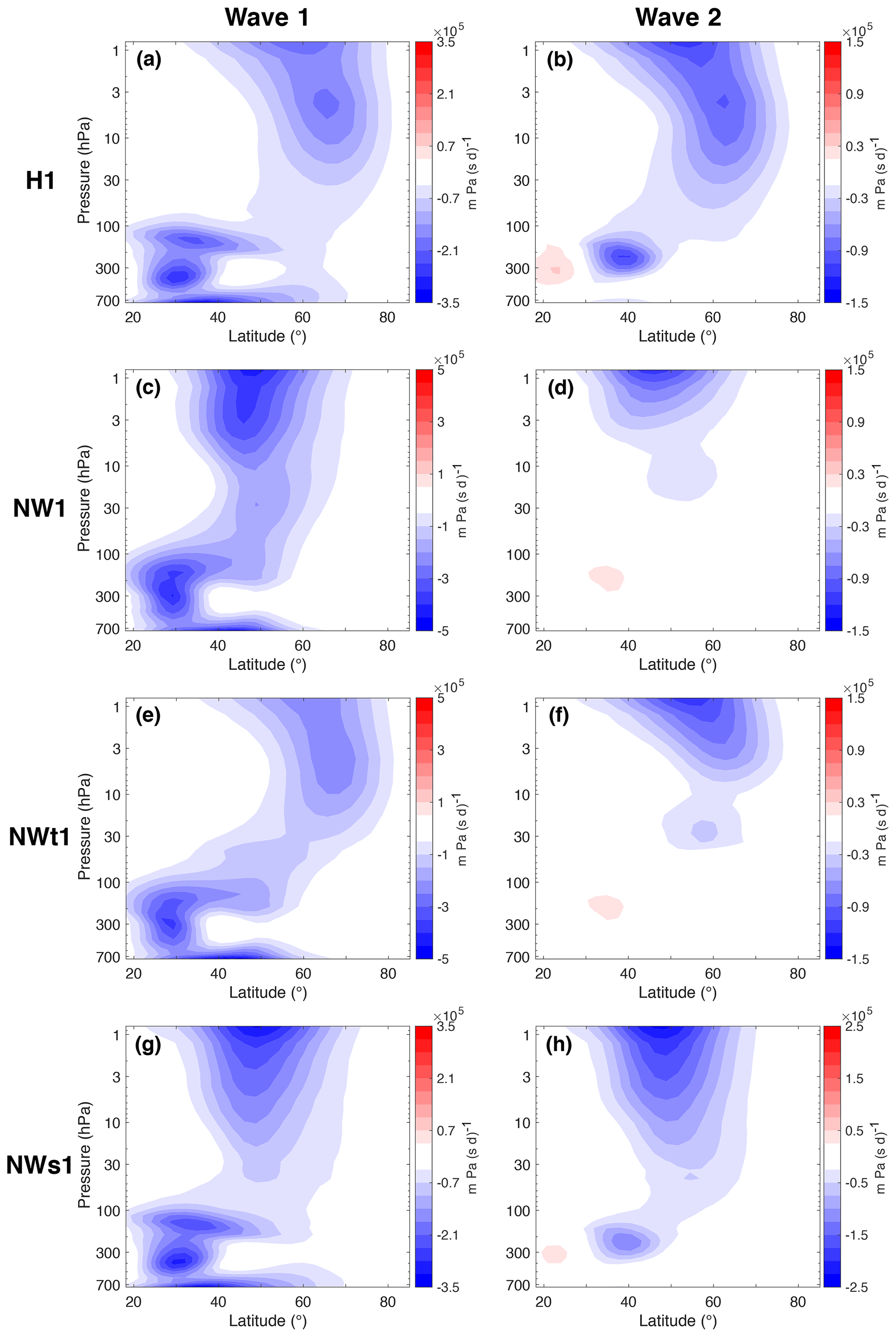
http://www.weather-clim-dynam.net/1/93/2020/wcd-1-93-2020-f05

Figure 5Vertical component of EP flux (F_p) for H1 (a, b), NW1 (c, d), NWt1 (e, f) and NWs1 (g, h). (a, c, e, g) Wave 1 components. (b, d, f, h) Wave 2 components. Values are scaled by p₀∕p, where p₀=1000 hPa. Contour intervals are 35 (a, g), 15 (b, d, f), 50 (c, e) and 25 (h) (in km Pa (s d)⁻¹).

Download

In contrast to the runs with wave 1 forcing, removal of WWIs in the troposphere and lower stratosphere does not significantly alter the SSW frequency when wave 2 forcing is used: NW2 and NWt2 have SSW frequencies of 0.51 and 0.45 compared to 0.48 in the control run. This is not surprising, considering the fact that almost all tropospheric and lower-stratospheric wave forcing in H2 is in the wave number of the forcing (Fig. 6), so removal of WWIs does not affect the climatological forcing as strongly as when wave 1 forcing is used. However, when WWIs are removed in the middle and upper stratosphere only (NWs2) the SSW frequency increases by 37 % compared to H2. The differences between this frequency and those of H2, NW2 and NWt2 are statistically significant. This increase in SSW frequency could be the reason for the weakened climatological polar night jet seen in Fig. 2c, although another explanation is that removal of WWIs weakens the polar night jet. This weakened jet would then require less wave forcing to create SSWs, which would increase the SSW frequency. Like the case of the mixed runs with wave 1 forcing, the increase in SSW frequency shows that middle- and upper-stratospheric WWIs play a major role in SSW generation. Interestingly, this change in SSW frequency is completely different from the one between NW1 and NWs1: with wave 2 forcing the SSW frequency increases without WWIs in the middle and upper stratosphere, while the opposite is true with wave 1 forcing.

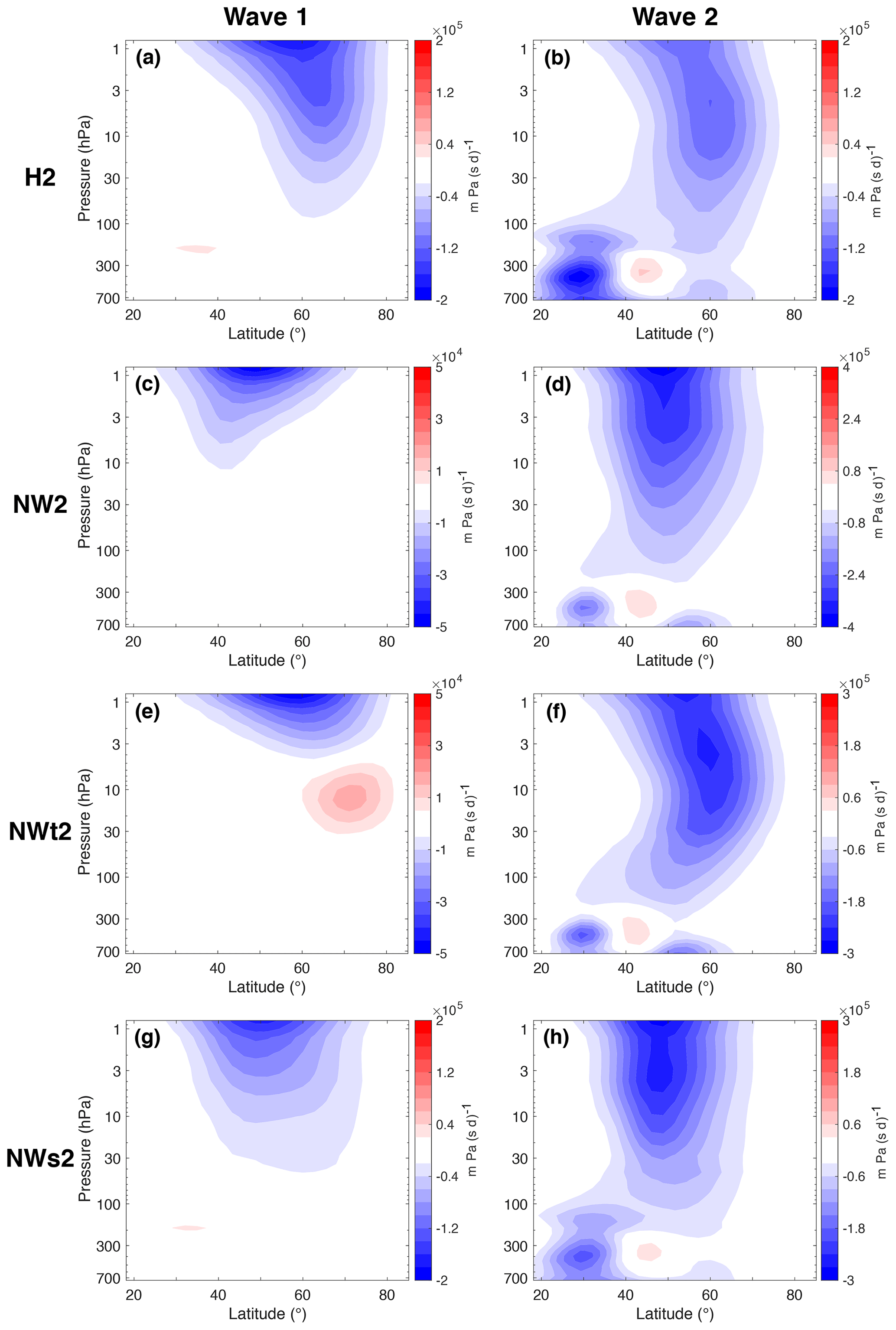
http://www.weather-clim-dynam.net/1/93/2020/wcd-1-93-2020-f06

Figure 6Vertical component of EP flux (F_p) for H2 (a, b), NW2 (c, d), (e, f) and NWs2 (g, h). (a, c, e, g) Wave 1 components. (b, d, f, h) Wave 2 components. Values are scaled by p₀∕p, where p₀=1000 hPa. Contour intervals are 20 (a, b, g), 5 (c, e), 40 (d) and 30 (f, h) (in km Pa (s d)⁻¹).

Download

Unlike the SSW frequencies, some changes in mean polar vortex strength and variability, as measured by the standard deviation of polar vortex strength, are consistent for model runs with both wave 1 and wave 2 forcing. In both cases the standard deviation of polar vortex strength is highest in the control run (H1 and H2) and lowest when WWIs are removed in the troposphere and lower stratosphere (NWt1 and NWt2). As can be expected, low mean polar vortex strengths and high standard deviations are correlated with high SSW frequencies. More revealing than these numbers are the time evolutions of polar vortex strength, seen in Fig. 7 for all eight model runs during 2000 d of the model simulations. The 2000 d are typical for the model runs. The data were smoothed with a 10 d filter for clarity, and Fig. S2 in the Supplement shows the same data unfiltered. Figure 7a shows how removal of WWIs affects the time evolution of the polar vortex strength when wave 1 heating is used. The strength of the polar vortex is highly variable in H1 (black) and has maximum and minimum strengths higher and lower than any of the other three model runs. Table 1 indicated that the polar vortex strength in NW1 (red) is both lower and less variable than H1, and Fig. 7a confirms this. The variations also seem to be of shorter duration in NW1 compared to H1. Based on the figure, the polar vortex strength in NWs1 (blue) is much more similar to that in H1 than to the one in NW1. The polar vortex in NWs1 exhibits the same long-term variability as H1 but does not become strongly negative as frequently as the one in H1. In Fig. 7a the polar vortex in NWt1 (green) exhibits little variability. From the figure it may seem like SSWs are infrequent in NWt1 compared to the other model runs, but it actually has a higher SSW frequency than NWs1. Instead, the polar vortex NWt1 exhibits a lot of short-term variability that is filtered out in Fig. 7a but visible in Fig. S2a.

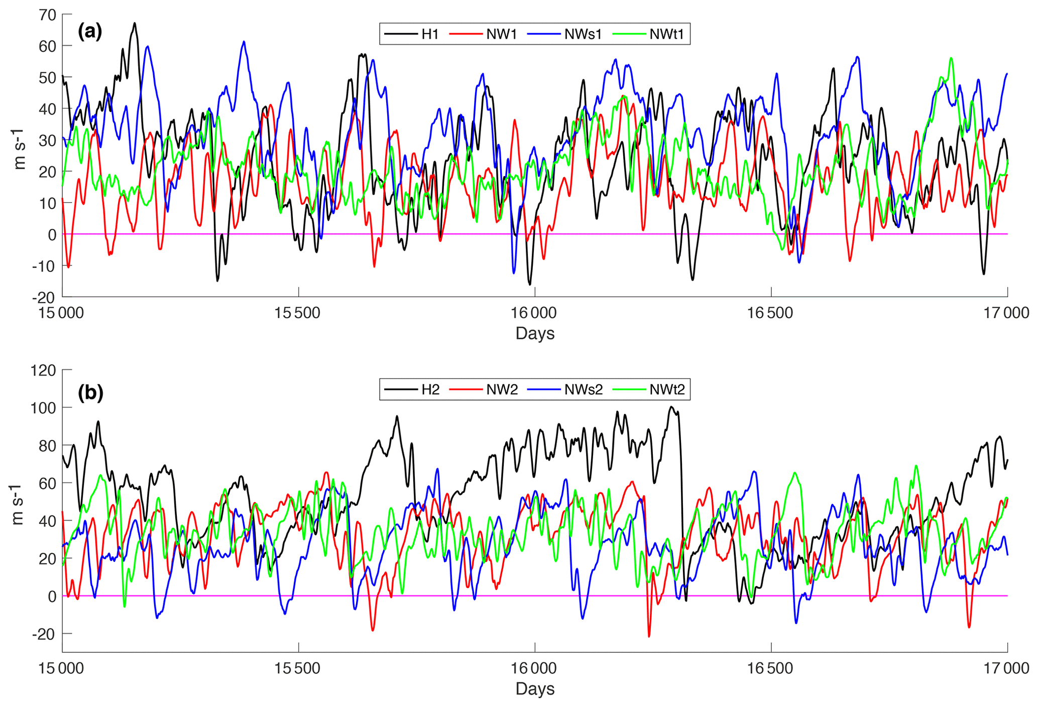
http://www.weather-clim-dynam.net/1/93/2020/wcd-1-93-2020-f07

Figure 7Zonal-mean zonal wind at 10 hPa and 60^∘ N for H1 and H2 (black), NW1 and NW2 (red), NWs1 and NWs2 (blue), and NWt1 and NWt2 (green) for model runs with wave 1 (a) and wave 2 (b) heating. The data were smoothed with a 10 d filter. The magenta line marks 0 m s⁻¹.

Download

The latitude of maximum polar vortex strength changes slightly between the model runs (from about 63 to 71^∘ N; see Figs. 2 and S1), and the relative mean values and variabilities in polar vortex strength therefore change when the latitude of interest is changed. However, the timescales of variability are qualitatively similar for given model runs with modest changes in latitude and pressure. Figures 7 and S2 can therefore be thought of as reasonable representations of overall polar vortex behavior.

As in the case of H1, the polar vortex strength in H2 has a larger variability than in any of the model runs with WWIs removed (Fig. 7b). The polar vortex strength in H2 varies on timescales up to 1000 d – much longer than any other model runs. As in the case of NW1 and H1, the polar vortex in NW2 has a lower mean strength and lower variability than that in H2, and the timescale of the variability is much shorter than in H2. Unlike the case with wave 1 heating, the polar vortex in NWs2 has a mean strength and variability that resembles that of NW2 more than that of H2. Just like in the case of NWt1, the variability in polar vortex strength in NWt2 is low, and much of the variability happens on short timescales which are filtered away in Fig. 7. However, unlike the case of NWt1 the polar vortex strength in NWt2 does not seem to vary on long timescales.

Figure 7 tells us much about how WWIs affect polar vortex strength and, by extension, SSW frequencies. The structure of the polar vortex variability in NWs1 is similar to that of H1, indicating that WWIs in the troposphere and lower stratosphere are important for much of the long-term (a few hundred days) variability in polar vortex strength when wave 1 heating is used. The fact that the SSW frequency is much lower in NWs1 compared to H1 could indicate that middle- and upper-stratospheric WWIs are important in order to strongly disturb the polar vortex, at least when the lower-stratospheric wave forcing is obtained with wave 1 heating in the presence of WWIs. The similarities in polar vortex behavior between NW2 and NWs2, on the other hand, indicate that WWIs in the troposphere and lower stratosphere are not as important when it comes to variability in the polar vortex (although the SSW frequency is higher in NWs2 compared to NW2). This is likely due to the fact that most of the tropospheric wave forcing in all model runs with wave 2 heating is in wave 2 (Fig. 6). This is not the case with wave 1 heating, where the tropospheric wave forcing has substantial wave 1 and wave 2 components in H1 and NWs1 but not NW1 and NWt1 (Fig. 5). The differences between H2 and NWs2 show that WWIs in the middle and upper stratosphere are crucial in setting the long-term behavior of the polar vortex when wave 2 heating is used. WWIs seem to strongly alter the structure of the stratosphere, which may alter the amount of wave forcing that can propagate up from below. The fact that the polar vortices in NWt1 and NWt2 exhibit the lowest amounts of variability, and variability on the shortest timescales, could indicate that much of any anomalous tropospheric and lower-stratospheric wave flux is damped away in the transition region between 50 and 30 hPa. Comparisons of total EP flux convergence (not shown) support this: compared to NW1 and NW2, there is stronger EP flux convergence in the transition region of NWt1 and NWt2 and less EP flux convergence further up in the stratosphere. The wave convergence in the transition region could produce low-frequency variability in the polar vortex strength and leave less wave flux to converge further up in the stratosphere, where it would likely affect the polar vortex more strongly.

Table 1 also contains the numbers and fractions of splits in the model runs; 59 % of SSWs in H1 are splits, and this number is increased to 80 % in NWt1 (a statistically significant difference). This result seems counterintuitive: as was mentioned above there is strong climatological tropospheric wave 1 and wave 2 flux in H1, while the tropospheric forcing is almost pure wave 1 when WWIs are not allowed. A possible explanation for this is that much of the wave activity is transferred from wave 1 to wave 2 in the upper stratosphere, where WWIs are allowed. Figure 3e and f show the wave 1 and wave 2 EP flux divergence for NWt1. The panels show that while the EP flux convergence in the upper stratosphere is certainly dominated by the wave 1 component (Fig. 3e), much of this wave 1 convergence is overlapped by large wave 2 divergence (Fig. 3f). These areas, which can be found above the transition region, likely show regions of energy transfer from wave 1 to wave 2. This energy transfer could supply enough wave 2 forcing to produce splits. The wave 2 vertical flux and flux convergence is lower than its wave 1 counterparts, which shows that the split and displacement ratios are not simply results of the relative climatological forcings. Another explanation for the wave 2 structures is that they arise through barotropic instability, which has been shown to induce wave 2 growth in the stratosphere. Hartmann (1983) investigated the barotropic instability of the polar night jet and suggested that the presence of wave 1 forcing may enhance the growth rates of shorter waves of similar phase speeds. Motivated by observations of wave 2 growth confined to the Southern Hemisphere winter stratosphere, Manney et al. (1991) investigated the possibility of barotropic instability as a mechanism for wave 2 growth using a barotropic model as well as a zonally symmetric three-dimensional model. They found that both wave 2 and 3, but in particular wave 2, were destabilized when the basic flow in the barotropic model contained stationary wave 1 and zonal flow. Unstable modes of wave 1, 2 and 3 were found in the three-dimensional model, and the authors noted that the wave 2 modes were usually the most unstable. To verify that barotropic instability could be the reason for the presence of wave 2 structures in these model runs, we calculated the quasi-geostrophic potential vorticity in the 20 to 90^∘ N region of the stratosphere. A condition for barotropic instability is that the meridional derivative of potential vorticity changes sign in the domain (Charney and Stern, 1962), and this condition is fulfilled for the absolute majority of days in all eight model runs.

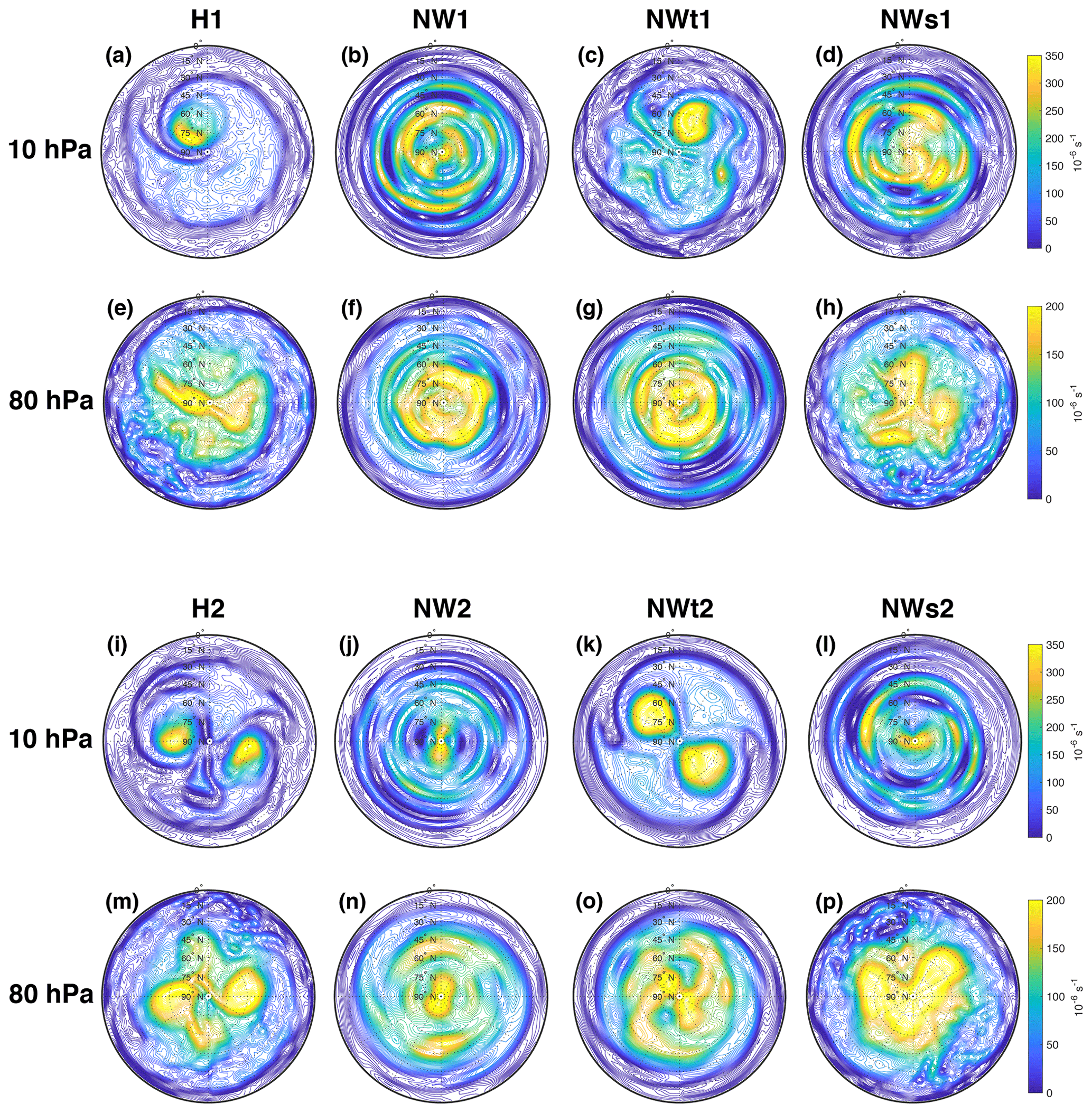
http://www.weather-clim-dynam.net/1/93/2020/wcd-1-93-2020-f08

Figure 8Absolute vorticity at 10 and 80 hPa on the central dates of an SSW with wave 1 heating (a–h) and wave 2 heating (i–p). Displacements can be seen in (a) and (c), while (i) and (k) show splits.

Download

The fractions of splits for NW1, NWs1, NW2 and NWs2 are in brackets to signify that the SSWs in these runs do not look like typical splits and displacements even though our SSW classification sorts these SSWs into one of the two categories. Figure 8 shows the absolute vorticity at 10 and 80 hPa on the central dates of typical SSWs in the eight model runs. Corresponding videos showing 60 d surrounding the SSWs can be found in the Supplement. The 10 hPa level is of interest, since that is where SSWs are usually defined, and the 80 hPa level was chosen because it is below the transition region. Figure 8a and e show a displacement in H1. The displacement of the polar vortex from the pole can clearly be seen at 10 hPa, while there is little to no suggestion of a displacement at 80 hPa. A clear split in H2 can be seen in Fig. 8i and m, and the split of the vortex extends all the way down to the lower stratosphere. In contrast, the 10 hPa levels in NW1, NWs1, NW2 and NWs2 (Fig. 8b, d, j and l) do not show either splits or displacements even though wave 1 and wave 2 zonal structures can be seen. Instead it seems that SSWs are followed by meridionally oriented waves when the effects of zonal WWIs are removed. These structures arise when the meridional shear of the flow $\partial u / \partial ϕ$ interacts with zonal wave numbers. Even though these are wave–wave interactions they are allowed to occur, since our method only removes interactions between zonal waves. Shepherd (1987) argued that interactions between stationary and transient waves in the observed atmosphere could be understood to first order through processes like these, where meridional shear transfers enstrophy along lines of constant zonal wave numbers. We have not investigated the effects of the polar meridional waves on the dynamics in these model runs, but we think it is unlikely that they have a significant effect on the overall climatology, since they only occur during vortex breakdowns and not when the vortex is less disturbed.

Even though typical splits and displacements do not occur when WWIs are not allowed in the middle and upper stratosphere, SSWs in NW1, NWs1, NW2 and NWs2 are still classified as “splits” and “displacements”, since the SSW classification of Lindgren et al. (2018) is based on wave amplitudes of geopotential height. The numbers in brackets in Table 1 therefore show that wave 2 amplitudes completely dominate SSWs when wave 2 forcing is used, with NW2 and NWs2 producing 100 % and 90 % wave 2-dominated SSWs (“splits”; statistically significant increases compared to H2). These numbers can be explained by the fact that most of the stratospheric wave flux is of wave 2: the upper stratospheric wave 2 flux in NW2 is an order of magnitude stronger than its wave 1 counterpart (Fig. 6c and d), and although the differences are not as large in NWs2, wave 2 forcing still dominates (Fig. 6g and h). Just like H1 and NWt1, SSWs with wave 1 forcing are also mostly wave 2-dominated, with 57 % and 80 % “splits” for NW1 and NWs1; the difference between the two is statistically significant. As in the case of NWt1, this cannot be explained by the dominant wave number of the stratospheric wave flux, since wave 1 is the dominant wave number (Fig. 5c, d, g and h). The fact that NW1 produces mostly wave 2-dominated events even though the tropospheric forcing is wave 1 and WWIs are not allowed suggests that enhanced growth of wave 2 in the presence of wave 1 forcing through barotropic instability, as hypothesized by Hartmann (1983) and shown by Manney et al. (1991), could be a major factor in the wave 2 structures seen in the wave 1 runs.

Figure 8 also shows that WWIs are only needed locally for typical splits and displacements to form. First, true splits and displacements do not occur in NWs1 or NWs2 even though the 80 hPa structures look similar to those of the control runs (Fig. 8e and m compared to h and p). As has already been established, the climatological tropospheric and lower-stratospheric wave forcing is very similar between these two runs. Second, NWt1 and NWt2 show that splits and displacements do occur when WWIs are removed in the troposphere and lower stratosphere, just as long as WWIs are allowed above. The structures of the 80 hPa levels in NW1 and NWt1 (Fig. 8f and g) as well as NW2 and NWt2 (Fig. 8n and o) are very similar, while the 10 hPa levels (Fig. 8b versus c and j versus k) are completely different, with NWt1 producing a displacement and NWt2 a split.

The fraction of splits in H2 was 74 %. When the effects of WWIs are removed in the troposphere and lower stratosphere (NWt2) the model only produces splits. While almost all climatological tropospheric F_p in H2 is in wave 2, the small amount of wave 1 that does exist (Fig. 6a) is apparently enough to make about every fourth SSW a displacement. Without WWIs in the troposphere and lower stratosphere this low-level wave 1 forcing disappears (Fig. 6e). There is almost no climatological wave 1 EP flux convergence in NWt2 (Fig. 4e), suggesting that there is very little wave 1–mean flow interaction.

5 Discussion and conclusions

In this paper we have investigated the effects of WWIs on SSW formation in an idealized GCM and found that removal of WWIs can change the SSW frequency dramatically. While SSWs can be considered wave–mean flow interactions to first order, our results show that removing or adding WWIs alters the conditions for SSW generation in non-predictable ways. While removing WWIs everywhere and below 50 hPa with wave 2 forcing (NW2 and NWt2) does not change the SSW frequency drastically, removal of WWIs in the upper stratosphere only (NWs2) increases the SSW frequency by 37 % compared to the control run. Since we showed that the wave forcing and climatology of the troposphere and lower stratosphere were dependent on whether or not WWIs were allowed in that same region, this 37 % increase can be attributed entirely to changes in nonlinear interactions in the upper stratosphere. The SSW frequencies with wave 1 forcing are strongly dependent on WWIs: even though H1 and NWs1 as well as NW1 and NWt1 have almost identical tropospheric and lower-stratospheric wave forcings their SSW frequencies are very different, with a 53 % decrease in NWs1 compared to H1 and a 45 % decrease in NWt1 compared to NW1. The results from these mixed runs can be contrasted to previous work which has emphasized the importance of tropospheric and lower-stratospheric wave flux for SSW generation (Polvani and Waugh, 2004; Birner and Albers, 2017). The results in this paper confirm previously published results showing that the upper stratosphere is not a passive recipient of tropospheric and lower-stratospheric wave forcing (Hitchcock and Haynes, 2016) and that stratospheric nonlinear processes are important for SSW generation (O'Neill and Pope, 1988).

While previous authors have investigated the effects of nonlinear interactions in stratospheric dynamics and found them to be important, this work is the first that has explicitly investigated the effects of WWIs on SSW frequencies in a global primitive-equation model. We find that removal of WWIs does not simply increase or decrease the SSW frequency: even with the same tropospheric forcing, removal of WWIs in the upper stratosphere can decrease SSW frequencies (H1 compared to NWs1) or increase it (NW1 compared to NWt1). To better understand the effects of WWIs on the polar vortex we also investigated the variability in polar vortex strength. We find that WWIs in the troposphere and lower stratosphere determine much of the long-term stratospheric polar vortex variability when wave 1 heating is used. In contrast, WWIs in the troposphere and lower stratosphere have a small impact on polar vortex variability when wave 2 heating is used, while middle- and upper-stratospheric WWIs are crucial in determining the long-term variability in polar vortex strength. Furthermore, the model runs where WWIs are removed in the troposphere and lower stratosphere but allowed above (NWt1 and NWt2) produce high-frequency variability in polar vortex strength but little long-term variability. It seems that much of the wave forcing from below converges in the transition region between “no WWIs” and “WWIs allowed”, which could be the source of the high-frequency variability. The frequent dissipation of wave forcing at lower levels could result in less wave forcing in the middle and upper stratosphere, causing lower amounts of low-frequency variability in polar vortex strength.

Some changes caused by removing WWIs can be found in all model runs: the stratospheric vertical wave flux and wave flux convergence is further equatorward when WWIs are not allowed in the middle and upper stratosphere. This is not a result of a shift in the stratospheric polar vortex, since latitudinal changes in the polar night jet locations are small compared to the changes in wave flux. The equatorward shift is consistent with the results of Robinson (1988).

We showed that in the absence of WWIs, meridionally oriented waves are created in the polar stratosphere, and the vortex is not displaced and does not split. We also found that splits and displacements occur even when WWIs are not allowed in the troposphere and lower stratosphere, indicating that only middle- and upper-stratospheric WWIs are necessary for split or displacement formation. These results are in contrast to those of Lordi et al. (1980), who found realistic wave 1 patterns in polar stereographic geopotential height when they used wave 1 forcing without WWIs. This discrepancy comes from the difference in methods used to remove the effects of WWIs: many authors, including Lordi et al. (1980), used zonal truncation to only allow one wave number to interact with the mean flow, while we removed all zonal WWIs. The meridional waves arise from interactions between the meridional shear of the flow and zonal wave numbers. Lordi et al. (1980) therefore found that wave 1–mean flow interactions are enough to create a displacement in the polar region, while we find that removing WWIs results in SSWs that are neither splits nor displacements. We do not believe that these meridional waves significantly affect the climatology of the model runs, since the waves only occur during vortex breakdowns.

With wave 2 forcing, all SSWs were splits when WWIs were turned off in the troposphere and lower stratosphere (NWt2). This is likely due to the fact that all tropospheric forcing is in wave 2 when WWIs are turned off in the lower levels, and the resulting SSWs are therefore splits. Even though splits and displacements do not occur without WWIs in the middle and upper stratosphere the SSWs in these model runs are still dominated by zonal wave 1 or wave 2 geopotential height anomalies. SSWs are strongly dominated by wave 2 anomalies in NW2 and NWs2, with 100 % and 90 % wave 2-dominated SSWs (“splits”). As in the case of NWt2, this can be explained by the fact that the stratospheric wave flux is mostly of wave 2 format in these model runs. The fraction of splits increased when WWIs were turned off in the lower levels with wave 1 forcing: 80 % splits in NWt1 compared to 59 % in H1. This is despite the fact that there is strong climatological tropospheric wave 1 and wave 2 wave flux in H1, while the flux is almost purely wave 1 in NWt1. The wave 2 forcing required to produce these splits could originate in the transition region between “no WWIs” and “WWIs allowed”, where some of the wave 1 flux is transferred to wave 2. Barotropic instability is also likely a factor: Hartmann (1983) suggested and Manney et al. (1991) demonstrated that waves of zonal wave number 1 may enhance growth rates of shorter waves. The strong wave 1 forcing in the lower stratosphere of NWt1 could make the flow unstable to wave 2, which would contribute to the large number of splits. SSWs in NW1 and NWs1 are also mostly wave 2-dominated, with 59 % and 80 % “splits” even though the stratospheric wave flux is mostly wave 1. The fact that NW1 produces wave 2-dominated events even though the forcing is of wave 1 and WWIs are not allowed strongly suggests that barotropic instability could be responsible for the wave 2 structure around SSWs in this model run. The precise nature of interactions between waves 1 and 2 in setting stratospheric variability is the subject of an ongoing investigation.

Code availability

The Flexible Modeling System (FMS) that is used in this paper can be found at: https://www.gfdl.noaa.gov/fms/ (GFDL, 2020).

Data availability

Zonal-mean zonal winds, geopotential height wave amplitudes, and 10 and 80 hPa absolute vorticity fields are archived at: https://doi.org/10.17605/OSF.IO/PR63B (Lindgren, 2018).

Supplement

The supplement related to this article is available online at: https://doi.org/10.5194/wcd-1-93-2020-supplement.

Video supplement

Videos of the SSWs seen in Fig. 8 are archived at: https://doi.org/10.17605/OSF.IO/3VRME (Lindgren, 2019).

Author contributions

EAL performed the simulations and data analysis and wrote the initial drafts of the paper. AS originated the idea for the project, contributed to the interpretation of the results and improved the final paper.

Competing interests

The authors declare that they have no conflict of interest.

Acknowledgements

We thank Paul O’Gorman, Edwin Gerber, Alan Plumb and Paul Kushner for useful discussions.

Financial support

This research has been supported by the Office of Graduate Education at the Massachusetts Institute of Technology (Donald O'Brien 2016–2017 Fellowship), the National Aeronautics and Space Administration (grant no. NNX13AF80G), the Simons Foundation (Junior Fellow award 354584), and NSF grant no. AGS-1921409 to Stanford University.

Review statement

This paper was edited by Thomas Birner and reviewed by two anonymous referees.

References

Allen, D. R., Bevilacqua, R. M., Nedoluha, G. E., Randall, C. E., and Manney, G. L.: Unusual stratospheric transport and mixing during the 2002 Antarctic winter, Geophys. Res. Lett., 30, 1599, https://doi.org/10.1029/2003GL017117, 2003. a

Austin, J. and Palmer, T. N.: The importance of nonlinear wave processes in a quiescent winter stratosphere, Q. J. Roy. Meteor. Soc., 110, 289–301, https://doi.org/10.1002/qj.49711046402, 1984. a, b

Baldwin, M. P. and Dunkerton, T. J.: Stratospheric Harbingers of Anomalous Weather Regimes, Science, 294, 581–584, https://doi.org/10.1126/science.1063315, 2001. a

Birner, T. and Albers, J. R.: Sudden Stratospheric Warmings and Anomalous Upward Wave Activity Flux, SOLA, 13, 8–12, https://doi.org/10.2151/sola.13A-002, 2017. a, b, c, d, e, f, g, h, i

Butler, A. H., Seidel, D. J., Hardiman, S. C., Butchart, N., Birner, T., and Match, A.: Defining Sudden Stratospheric Warmings, B. Am. Meteorol. Soc., 96, 1913–1928, https://doi.org/10.1175/BAMS-D-13-00173.1, 2015. a

Charlton, A. J. and Polvani, L. M.: A New Look at Stratospheric Sudden Warmings. Part I: Climatology and Modeling Benchmarks, J. Climate, 20, 449–469, https://doi.org/10.1175/JCLI3996.1, 2007. a, b, c, d, e

Charney, J. G. and Drazin, P. G.: Propagation of Planetary-Scale Disturbances from the Lower into the Upper Atmosphere, J. Geophys. Res., 66, 83–109, https://doi.org/10.1029/JZ066i001p00083, 1961. a

Charney, J. G. and Stern, M. E.: On the Stability of Internal Baroclinic Jets in a Rotating Atmosphere, J. Atmos. Sci., 19, 159–172, https://doi.org/10.1175/1520-0469(1962)019<0159:OTSOIB>2.0.CO;2, 1962. a

Chemke, R. and Kaspi, T.: The Effect of Eddy-Eddy Interactions on Jet Formation and Macroturbulent Scales, J. Atmos. Sci., 73, 2049–2059, https://doi.org/10.1175/JAS-D-15-0375.1, 2016. a, b, c

Constantinou, N. C., Farrell, B. F., and Ioannou, P. J.: Emergence and Equilibration of Jets in Beta-Plane Turbulence: Applications of Stochastic Structural Stability Theory, J. Atmos. Sci., 71, 1818–1842, https://doi.org/10.1175/JAS-D-13-076.1, 2014. a

de la Cámara, A., Birner, T., and Albers, J. R.: Are Sudden Stratospheric Warmings Preceded by Anomalous Tropospheric Wave Activity?, J. Climate, 32, 7173–7189, https://doi.org/10.1175/JCLI-D-19-0269.1, 2019. a, b

Edmon Jr., H. J., Hoskins, B. J., and McIntyre, M. E.: Eliassen-Palm Cross Sections for the Troposphere, J. Atmos. Sci., 37, 2600–2616, https://doi.org/10.1175/1520-0469(1980)037<2600:EPCSFT>2.0.CO;2, 1980. a

Gerber, E. P. and Polvani, L. M.: Stratosphere-Troposphere Coupling in a Relatively Simple AGCM: The Importance of Stratospheric Variability, J. Climate, 22, 1920–1933, https://doi.org/10.1175/2008JCLI2548.1, 2009. a, b

GFDL: Flexible Modeling System (FMS), available at: https://www.gfdl.noaa.gov/fms/, last access: 27 February 2020. a

Hartmann, D. L.: Barotropic Instability of the Polar Night Jet Stream, J. Atmos. Sci., 40, 817–835, https://doi.org/10.1175/1520-0469(1983)040<0817:BIOTPN>2.0.CO;2, 1983. a, b, c

Held, I. M. and Suarez, M. J.: A Proposal for the Intercomparison of the Dynamical Cores of Atmospheric General Circulation Models, B. Am. Meteorol. Soc., 75, 1825–1830, https://doi.org/10.1175/1520-0477(1994)075<1825:APFTIO>2.0.CO;2, 1994. a

Hitchcock, P. and Haynes, P. H.: Stratospheric control of planetary waves, Geophys. Res. Lett., 43, 11884–11892, https://doi.org/10.1002/2016GL071372, 2016. a, b, c, d

Holton, J. R. and Mass, C.: Stratospheric Vacillation Cycles, J. Atmos. Sci., 33, 2218–2225, https://doi.org/10.1175/1520-0469(1976)033<2218:SVC>2.0.CO;2, 1976. a, b

Lindgren, E. A.: Data for “The Role of Wave-Wave Interactions in Sudden Stratospheric Warming Formation”, https://doi.org/10.17605/OSF.IO/PR63B, 2018 (updated 2020). a

Lindgren, E. A.: Supplemental movies for “The Role of Wave-Wave Interactions in Sudden Stratospheric Warming Formation”, https://doi.org/10.17605/OSF.IO/3VRME, 2019 (updated 2020). a

Lindgren, E. A., Sheshadri, A., and Plumb, R. A.: Sudden Stratospheric Warming Formation in an Idealized General Circulation Model Using Three Types of Tropospheric Forcing, J. Geophys. Res.-Atmos., 123, 10125–10139, https://doi.org/10.1029/2018JD028537, 2018. a, b, c, d, e, f, g, h, i, j, k, l, m, n, o, p, q

Lordi, N. J., Kasahara, A., and Kao, S. K.: Numerical Simulation of Stratospheric Sudden Warmings with a Primitive Equation Spectral Model, J. Atmos. Sci., 37, 2746–2767, https://doi.org/10.1175/1520-0469(1980)037<2746:NSOSSW>2.0.CO;2, 1980. a, b, c, d, e

Manney, G. L., Elson, L. S., Mechoso, C. R. and Farrara, J. D.: Planetary-Scale Waves in the Southern Hemisphere Winter and Early Spring Stratosphere: Stability Analysis, J. Atmos. Sci., 48, 2509–2523, https://doi.org/10.1175/1520-0469(1991)048<2509:PSWITS>2.0.CO;2, 1991. a, b, c

Martineau, P., Chen, G., Son, S.-W., and Kim, J.: Lower-Stratospheric Control of the Frequency of Sudden Stratospheric Warming Events, J. Geophys. Res.-Atmos., 123, 3051–3070, https://doi.org/10.1002/2017JD027648, 2018. a, b

Matsuno, T.: A dynamical model of the stratospheric sudden warming, J. Atmos. Sci., 28, 1479–1494, https://doi.org/10.1175/1520-0469(1971)028<1479:ADMOTS>2.0.CO;2, 1971. a

Matthewman, N. J., Esler, J. G., Charlton-Perez, A. J. and Polvani, L. M.: A New Look at Stratospheric Sudden Warmings. Part III: Polar Vortex Evolution and Vertical Structure, J. Climate, 22, 1566–1585, https://doi.org/10.1175/2008JCLI2365.1, 2009. a

Maycock, A. C. and Hitchcock, P.: Do split and displacement sudden stratospheric warmings have different annular mode signatures?, Geophys. Res. Lett., 42, 10943–10951, https://doi.org/10.1002/2015GL066754, 2015. a

Mitchell, D. M., Gray, L. J., Anstey, J., Baldwin, M. P., and Charlton-Perez, A. J.: The Influence of Stratospheric Vortex Displacements and Splits on Surface Climate, J. Climate, 26, 2668–2682, https://doi.org/10.1175/JCLI-D-12-00030.1, 2013. a

O'Gorman, P. A. and Schneider, T.: Recovery of atmospheric flow statistics in a general circulation model without nonlinear eddy-eddy interactions, Geophys. Res. Lett., 34, L22801, https://doi.org/10.1029/2007GL031779, 2007. a, b, c, d, e

O'Neill, A. and Pope, V. D.: Simulations of linear and nonlinear disturbances in the stratosphere, Q. J. Roy. Meteor. Soc., 114, 1063–1110, https://doi.org/10.1002/qj.49711448210, 1988. a, b, c, d

Polvani, L. M. and Kushner, P. J.: Tropospheric response to stratospheric perturbations in a relatively simple general circulation model, Geophys. Res. Lett., 29, 18-1–18-4, https://doi.org/10.1029/2001GL014284, 2002. a

Polvani, L. M. and Waugh, D. W.: Upward Wave Activity Flux as a Precursor to Extreme Stratospheric Events and Subsequent Anomalous Surface Weather Regimes, J. Climate, 17, 3548–3554, https://doi.org/10.1175/1520-0442(2004)017<3548:UWAFAA>2.0.CO;2, 2004. a, b, c, d, e, f

Robinson, W. A.: Irreversible Wave-Mean Flow Interactions in a Mechanistic Model of the Stratosphere, J. Atmos. Sci., 45, 3413–3430, https://doi.org/10.1175/1520-0469(1988)045<3413:IWFIIA>2.0.CO;2, 1988. a, b, c, d, e

Scott, R. K. and Polvani, L. M.: Stratospheric control of upward wave flux near the tropopause, Geophys. Res. Lett., 31, L02115, https://doi.org/10.1029/2003GL017965, 2004. a

Scott, R. K. and Polvani, L. M.: Internal variability of the winter stratosphere. Part I: Time-independent forcing, J. Atmos. Sci., 63, 2758–2776, https://doi.org/10.1175/JAS3797.1, 2006. a

Seviour, W. J. M., Mitchell, D. M., and Gray, L. J.: A practical method to identify displaced and split stratospheric polar vortex events, Geophys. Res. Lett., 40, 5268–5273, https://doi.org/10.1002/grl.50927, 2013. a

Shepherd, T. G.: A Spectral View of Nonlinear Fluxes and Stationary-Transient Interaction in the Atmosphere, J. Atmos. Sci., 44, 1166–1179, https://doi.org/10.1175/1520-0469(1987)044<1166:ASVONF>2.0.CO;2, 1987. a

Sheshadri, A., Plumb, R. A., and Gerber, E. P.: Seasonal Variability of the Polar Stratospheric Vortex in an Idealized AGCM with Varying Tropospheric Wave Forcing, J. Atmos. Sci., 72, 2248–2266, https://doi.org/10.1175/JAS-D-14-0191.1, 2015. a, b

Smith, A. K., Gille, J. C., and Lyjak, L. V.: Wave-Wave Interactions in the Stratosphere: Observations during Quiet and Active Wintertime Periods, J. Atmos. Sci., 41, 363–373, https://doi.org/10.1175/1520-0469(1984)041<0363:WIITSO>2.0.CO;2, 1983. a

Srinivasan, K., and Young, W. R.: Zonostrophic Instability, J. Atmos. Sci., 69, 1633–1656, https://doi.org/10.1175/JAS-D-11-0200.1, 2012. a

Tobias, S. M. and Marston, J. B.: Direct Statistical Simulation of Out-of-Equilibrium Jets, Phys. Rev. Lett., 110, 104502, https://doi.org/10.1103/PhysRevLett.110.104502, 2013. a

White, I., Garfinkel, C. I., Gerber, E. P., Jucker, M., Aquila, V., and Oman, L. D.: The Downward Influence of Sudden Stratospheric Warmings: Association with Tropospheric Precursors, J. Climate, 32, 85–108, https://doi.org/10.1175/JCLI-D-18-0053.1, 2019. a

Yoden, S.: An Illustrative Model of Seasonal and Interannual Variations of the Stratospheric Circulation, J. Atmos. Sci., 47, 1845–1853, https://doi.org/10.1175/1520-0469(1990)047<1845:AIMOSA>2.0.CO;2, 1990. a, b

Articles

Short summary

Sudden stratospheric warmings (SSWs) are extreme events that influence surface weather up to 2 months after onset. We remove wave–wave interactions (WWIs) in vertical sections of a general circulation model to investigate the role of WWIs in SSW formation. We show that the effects of WWIs depend strongly on the pressure levels where they occur and the zonal structure of the wave forcing in the troposphere. Our results highlight the importance of upper-level processes in stratospheric dynamics.