the Creative Commons Attribution 4.0 License.
the Creative Commons Attribution 4.0 License.
 | 26 Feb 2020
The substructure of extremely hot summers in the Northern Hemisphere
Matthias Röthlisberger
Michael Sprenger
Emmanouil Flaounas
Urs Beyerle
Heini Wernli
In the last decades, extremely hot summers (hereafter extreme summers) have challenged societies worldwide through their adverse ecological, economic and public-health effects. In this study, extreme summers are identified at all grid points in the Northern Hemisphere in the upper tail of the June–July–August (JJA) seasonal mean 2 m temperature (T2m) distribution, separately in ERA-Interim (ERAI) re-analyses and in 700 simulated years with the Community Earth System Model (CESM) large ensemble for present-day climate conditions. A novel approach is introduced to characterise the substructure of extreme summers, i.e. to elucidate whether an extreme summer is mainly the result of the warmest days being anomalously hot, of the coldest days being anomalously mild or of a general shift towards warmer temperatures on all days of the season. Such a statistical characterisation can be obtained from considering so-called rank day anomalies for each extreme summer – that is, by sorting the 92 daily mean T2m values of an extreme summer and by calculating, for every rank, the deviation from the climatological mean rank value of T2m.
Applying this method in the entire Northern Hemisphere reveals spatially strongly varying extreme-summer substructures, which agree remarkably well in the re-analysis and climate model data sets. For example, in eastern India the hottest 30 d of an extreme summer contribute more than 65 % to the total extreme-summer T2m anomaly, while the colder days are close to climatology. In the high Arctic, however, extreme summers occur when the coldest 30 d are substantially warmer than they are climatologically. Furthermore, in roughly half of the Northern Hemisphere land area, the coldest third of summer days contributes more to extreme summers than the hottest third, which highlights that milder-than-normal coldest summer days are a key ingredient of many extreme summers. In certain regions, e.g. over western Europe and western Russia, the substructure of different extreme summers shows large variability and no common characteristic substructure emerges. Furthermore, we show that the typical extreme-summer substructure in a certain region is directly related to the region's overall T2m rank day variability pattern. This indicates that in regions where the warmest summer days vary particularly strongly from one year to the other, these warmest days are also particularly anomalous in extreme summers (and analogously for regions where variability is largest for the coldest days). Finally, for three selected regions, thermodynamic and dynamical causes of extreme-summer substructures are briefly discussed, indicating that, for instance, the onset of monsoons, physical boundaries like the sea ice edge or the frequency of occurrence of Rossby wave breaking strongly determines the substructure of extreme summers in certain regions.
Please read the corrigendum first before continuing.
-
Notice on corrigendum
The requested paper has a corresponding corrigendum published. Please read the corrigendum first before downloading the article.
-
Article
(14066 KB)
- Corrigendum
-
Supplement
(377 KB)
-
The requested paper has a corresponding corrigendum published. Please read the corrigendum first before downloading the article.
- Article
(14066 KB) - Corrigendum
-
Supplement
(377 KB) - BibTeX
- EndNote


During the last decades, numerous high-impact hot-temperature extremes occurred on approximately seasonal timescales, including the extremely hot European summer in 2003 (Fink et al., 2004; Schär and Jendritzky, 2004), the 2010 Russian heat wave (Barriopedro et al., 2011), the hot and dry summer of 2015 in Europe (Dong et al., 2016; Hoy et al., 2017; Orth et al., 2016), the hot and humid summer of 2015 in western India and Pakistan (Wehner et al., 2016), and the concurrent heat waves across the Northern Hemisphere in the summer of 2018 (Vogel et al., 2019). It is well known that individual heat waves on timescales of up to a few weeks cause societal challenges, for example serious public-health issues (e.g. Fouillet et al., 2006). However, the large socio-economic and ecological impacts of the seasonal events listed above (e.g. Ciais et al., 2005; Buras et al., 2019) illustrated that many economic sectors such as agriculture, tourism and re-insurance are particularly susceptible to temperature extremes on seasonal (as opposed to synoptic) timescales. Therefore, understanding the statistical properties of entire extremely hot summers (hereafter referred to as “extreme summers”) as well as their physical causes is a research topic of high societal relevance.
The concept of an extreme summer is closely related to the concept of a heat wave, even though there are important differences. An individual heat wave is commonly understood to be a single, quasi-continuous episode of abnormally hot surface weather with a duration ranging from days to weeks (Russo et al., 2015; Zschenderlein et al., 2019). Heat waves are thus strongly influenced by individual synoptic flow features such as atmospheric blocks (Brunner et al., 2017; Pfahl and Wernli, 2012; Röthlisberger and Martius, 2019; Zschenderlein et al., 2019), stationary ridges (Sousa et al., 2018) or recurrent Rossby wave patterns (Röthlisberger et al., 2019). In contrast, extreme summers have a fixed duration (of 3 months), which is beyond the timescale of these synoptic flow features. Consequently, extreme summers require a temporal organisation of the relevant synoptic flow features, which can occur either “by chance” (internal atmospheric variability) or favoured by more slowly varying processes. Possible candidates for the latter are soil moisture fluctuations (Fischer et al., 2007; Lorenz et al., 2010; Seneviratne et al., 2010), sea ice dynamics (Cohen et al., 2014), or large-scale modes of variability in the ocean and atmosphere (e.g. Schneidereit et al., 2012). Understanding how this temporal organisation of weather within seasons occurs is challenging, as it requires a seamless approach (Hoskins, 2013), which couples weather system dynamics to these slower varying processes.
Like any other summer, an extreme summer will inevitably contain cooler and hotter days, which constitute the upper and lower parts of the daily mean 2 m temperature (T2m) distribution during that summer. However it is currently not known which part of the T2m distribution is particularly anomalous during an extreme summer. Thus, extreme summers with distinct “substructures” might occur, some of which are schematically illustrated in Fig. 1. For example, a summer might be an extreme summer because the hottest days of the season are particularly anomalous, with the remainder of the summer days being only moderately warmer than or even close to climatology. Such an extreme-summer substructure was observed in large parts of Europe in the summer of 2015, when the anomalies of the seasonal hottest days exceeded those of the seasonal mean by almost a factor of 2 (Dong et al., 2016). Hence the hottest days of the 2015 summer contributed overproportionately to the seasonal mean anomaly. However, also other substructures are plausible: a suppression of cool summer days, a uniform shift in the entire summer temperature distribution or any combination of these three options.
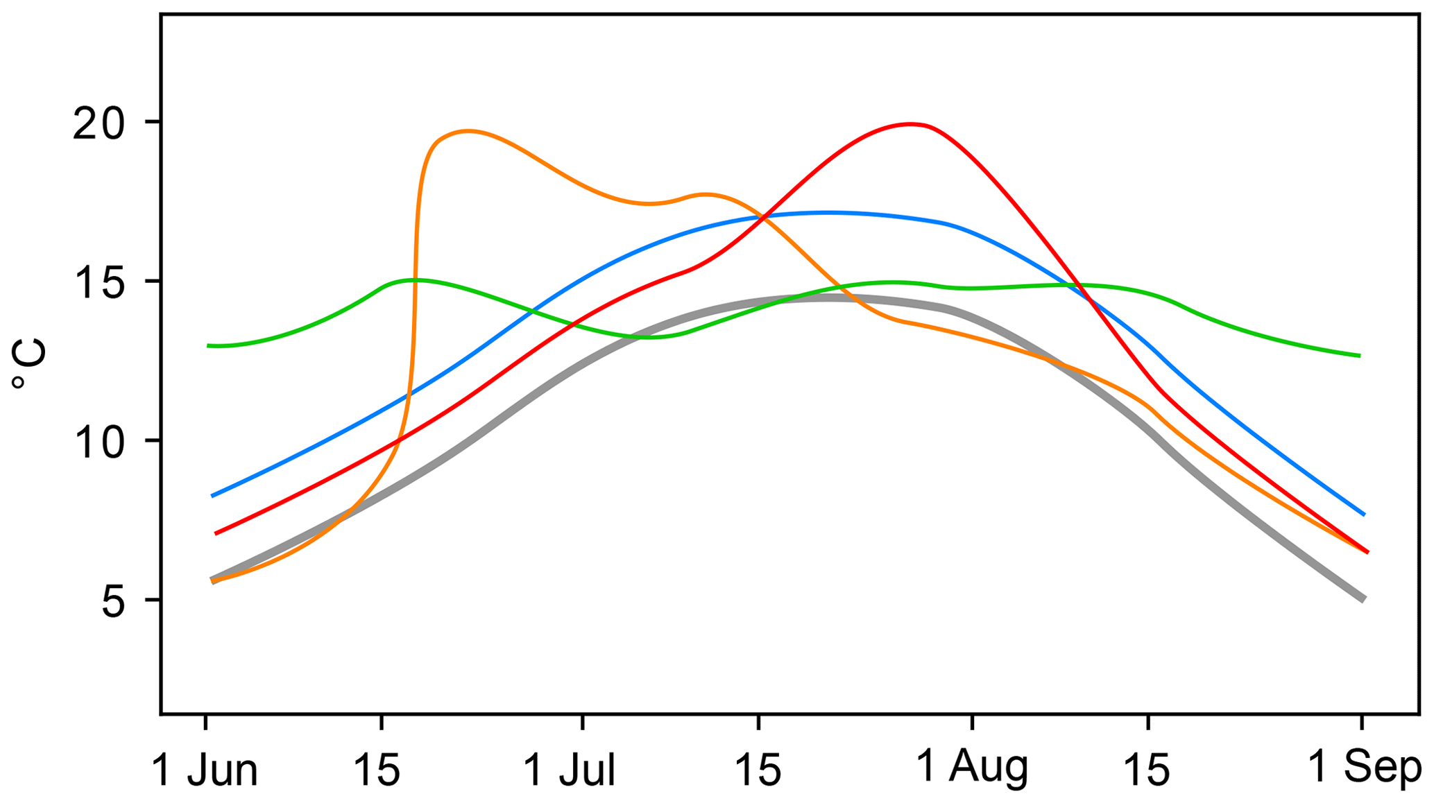
Figure 1Schematic surface temperature evolution during extreme summers with different substructures: an extreme summer arising from just one heat wave (orange), from a suppression of cool summer days (green), from a shift in the entire T2m distribution (blue) and from a general shift towards higher temperatures and a heat wave (red). The schematic climatological surface temperature evolution is depicted in grey.
Knowledge about the extreme-summer substructure is relevant for at least two reasons. Firstly, the societal impact of an extreme summer featuring one period (or several periods) of extremely hot temperatures (i.e. hottest summer days being hotter than normal) will likely differ from the societal impact of an extreme summer resulting primarily from a suppression of cool summer days (i.e. coldest summer days being milder than normal) or from an extreme summer characterised by a uniform shift in the entire temperature distribution (i.e. all summer days warmer than normal). Secondly, also the physical and meteorological causes of extreme summers with such distinct substructures conceivably differ. Thus, identifying the substructure of extreme summers is likely a starting point for understanding also their physical causes.
The purpose of this study is to characterise extreme summers statistically by quantifying their substructure. To do so, we define extreme summers in the upper tail of the June–July–August (JJA) mean 2 m temperature (T2m) distribution. Thereafter, the extreme-summer substructure is assessed by decomposing the seasonal mean T2m anomaly of a particular extreme summer into the contributions from all rank days of that season (i.e. the contribution from the coldest day, the second-coldest day, etc.). This decomposition thus allows quantifying the contributions from all parts of the T2m distribution (e.g. the coldest, middle and hottest thirds of summer days) to the seasonal T2m anomaly of an extreme summer.
Here we use the ERA-Interim (ERAI) re-analysis data set to study the substructure of past extreme summers. However, extreme summers are by definition extremely rare events. Thus, in order to yield robust results, a climatological investigation of the extreme-summer substructure requires much longer data records than provided by ERA-Interim or any other currently available high-quality re-analysis data set. We therefore complement ERA-Interim with a 700-year present-day climate simulation (for details, see Sect. 2.2) to address the following research goals:
-
Propose and illustrate a simple method for decomposing, at each grid point, the seasonal mean temperature anomaly into its contributions from each rank day.
-
Use this decomposition to analyse the substructure of extreme summers separately at selected grid points.
-
Quantify and compare the spatial variability in extreme-summer substructures in the Northern Hemisphere in both re-analysis and climate model data.
-
Illustrate physical causes of the observed (and simulated) extreme-summer substructures in selected regions.
2.1 ERA-Interim
We use ERA-Interim re-analysis data (Dee et al., 2011) covering the period 1979–2018. ERA-Interim is originally produced with a T255 spectral horizontal resolution and 60 hybrid σ–p levels in the vertical. We interpolated the data horizontally to a 1∘ by 1∘ grid and vertically to pressure and isentropic levels. The ERA-Interim data are provided at 6-hourly time intervals; in this study however, we aggregated all data to a daily temporal resolution. Besides the T2m fields, we also use potential vorticity (PV), total precipitation, 250 hPa meridional winds and sea ice concentration. Furthermore, we remove a (40-year) linear trend from all JJA T2m data at each grid point. Our analyses hereafter are based on the detrended data, except for Figs. 2, 8 and 9, which are more easily understood based on the non-detrended data (Figs. 2 and 8) or where the absolute T2m values are important (Fig. 9).
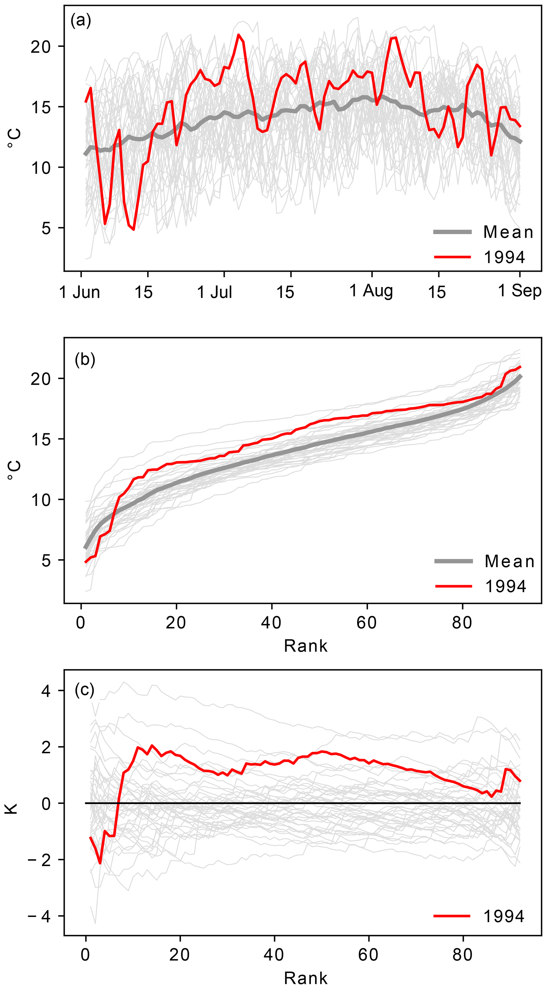
Figure 2Steps in computing values at the grid point closest to Zurich, Switzerland (47∘ N, 9∘ E). Values for the 1994 summer are highlighted in red. Panel (a) shows ERA-Interim T2m at 47∘ N, 9∘ E, for all 40 ERA-Interim summers. The sorted T2m values () are shown in panel (b) and the values in panel (c). Note that for illustrating purposes Fig. 2 presents non-detrended T2m data.
2.2 CESM
Besides ERA-Interim, the Community Earth System Model version 1 (CESM; Hurrell et al., 2013) is used to perform present-day climate simulations using restart files from the CESM large ensemble project (CESM-LE.; Kay et al., 2015). We use atmospheric fields at daily temporal resolution, with a horizontal resolution of approximately 1∘ and 30 vertical levels. The original CESM-LE data contain a 35-member ensemble of simulations started on 1 January 1920 and integrated forward in time until 2100. These 35 “macro-ensemble” members were rerun for the period from 1 January 1990 to 31 December 1999 in order to obtain temporally high-resolution three-dimensional model output. To further increase the number of simulated JJA seasons, a “micro-ensemble” with additional 35 members was initialized from member one of the macro-ensemble, on 1 January 1980, by adding an O(10−13) perturbation to the initial atmospheric temperature field of each micro-ensemble member. These additional micro-ensemble runs are then integrated forward in time until 31 December 1999. Fischer et al. (2013) have shown that at the latest after a decade, the micro-ensemble members exhibit a similar spread in atmospheric variables compared to members of the macro-ensemble. Thus, for the period 1990–1999, the micro-ensemble members can be regarded as additional independent members, yielding a total of 70 ensemble members covering the 10-year period from 1990 to 1999, i.e. 700 years of present-day climate. As for ERA-Interim data, a linear trend is removed from all JJA T2m data at each grid point and in each ensemble member. Note, however, that due to the ensemble set-up, this trend is calculated over only 10 years.
2.3 Decomposing a seasonal T2m anomaly to quantify the season's substructure
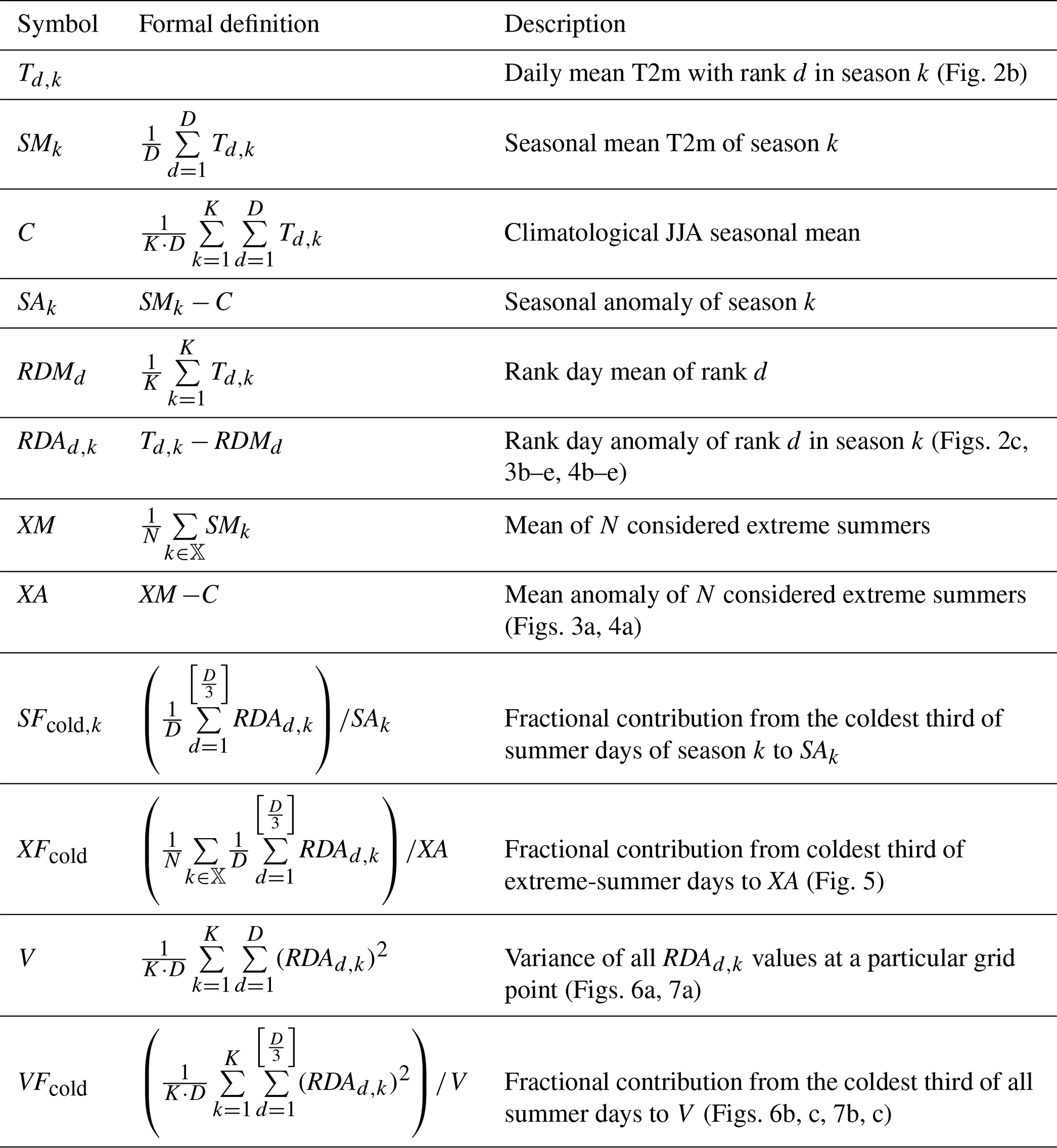
To examine the substructure of a particular July–August (JJA) season k, we decompose its seasonal T2m anomaly (SAk) into contributions from the ranked D daily T2m values of season k, where D is the number of days in season k (e.g. for JJA, D=92). We thus aim to quantify how much each rank day (i.e. coldest day, second-coldest day, etc.) of season k contributes to the seasonal anomaly SAk. This decomposition of SAk is illustrated for the example grid point 47∘ N, 9∘ E (near Zurich, Switzerland), in Fig. 2 and introduced more formally below. It is applied to both data sets separately in exactly the same fashion, and, therefore, a superscript M∈{ERAI,CESM} will only be used where it is necessary to explicitly distinguish between the two data sets. All the important statistical quantities used in this study are summarised in Table 1. Furthermore, bear in mind that all these quantities are calculated at each grid point individually.
Table 1Definitions and descriptions of important quantities used in this study.
We start by ranking all daily mean T2m values within their respective season k (Fig. 2a, b) and computing seasonal means (SMk), i.e.
where Td,k is the daily mean T2m value with rank d in season k (i.e. the temporal ordering of the days is lost; see Fig. 2b). At each grid point we thus compute KERAI=40 seasonal mean values for ERA-Interim and KCESM=700 values for CESM.
The climatological seasonal mean (C) is also calculated from the ranked daily mean T2m values (Td,k) as
Hereby, is the average T2m value of all K days with rank d in their respective season, e.g. for d=1 the average coldest day of the season and for d=92 the average hottest day of the season. Hence, C is computed as the mean over the average T2m values for each rank. These rank day T2m means (bold grey contour in Fig. 2b) are hereafter referred to as
Using the RDMd, the seasonal T2m anomaly of any season k (SAk) can be decomposed into contributions from each of the D rank days:
where in the last equality the rank day anomaly of the day with rank d in season k is introduced as . In other words, the seasonal mean anomaly SAk is expressed as the average rank day anomaly (see also Fig. 2c).
This decomposition of SAk thus allows assessing the exact contribution from each (ranked) day of season k to SAk. For example, if for a particular season k SAk=1 K and K (i.e, the hottest day of season k is 3 K warmer than the respective rank day mean) this day contributed K, or 3.26 %, to the seasonal anomaly SAk. In the following we split the 92 d of each JJA season k into three parts according to their rank and focus on the relative contributions to SAk from the coldest, middle and hottest third of the 92 d of season k by calculating
The notation [x] hereby stands for x rounded to the nearest integer. For computing contributions to SAk from the middle and hottest thirds of the summer days (SFmiddle,k and SFhot,k), the sum in Eq. (5) runs from to for SFmiddle,k and from to D for SFhot,k. By construction, the sum of the three fractions amounts to 1.
2.4 Identification and substructure of extreme summers
Extremely hot summers at each grid point in the Northern Hemisphere are identified in the ERA-Interim (CESM) data set as the five (35) hottest JJA seasons, yielding two sets of extreme summers, , M∈{ERAI,CESM}, with NERAI=5 and NCESM=35 members, respectively. Hence, ERA-Interim extreme summers correspond to the 12.5 % hottest summers (5 out of 40), while the CESM extreme summers correspond to the 5 % hottest summers (35 out of 700).
An analogous procedure to that described in Sect. 2.3 is employed to quantify the contributions from each of the three thirds of the extreme-summer days to the average T2m anomaly of the N considered extreme summers. The mean of these extreme summers (XM) is calculated as and is used to compute the mean anomaly of these extreme summers, . The relative contributions from the three thirds of the summer days to the extreme-summer anomaly XA are calculated as, for example,
The quantities XFcold, XFmiddle and XFhot again add up to 1 and quantify the relative contributions from the three thirds to the average T2m anomaly of all extreme summers at a particular grid point. Note that the quantities XFcold, XFmiddle and XFhot characterise the mean extreme-summer substructure at a particular grid point, while SFcold,k, SFmiddle,k and SFhot,k characterise the substructure of a single season k.
3.1 Extreme-summer T2m anomalies
Figures 3a and 4a depict the average T2m anomalies during extreme summers in the two data sets (XAERAI and XACESM, respectively). In both data sets, XA exhibits considerable spatial variability. The ERA-Interim extreme summers have temperature anomalies of up to 3 K over western Russia, while over some tropical ocean areas XAERAI is less than 0.5 K (Fig. 3a). The XACESM field exhibits a generally similar spatial pattern to XAERAI, with larger values over land than over the oceans (Fig. 4a). However, XACESM generally exceeds XAERAI, as the summers 𝕏CESM are statistically more extreme than the summers 𝕏ERAI. In the following, we decompose the extreme-summer T2m anomalies (XA) shown in Figs. 3a and 4a using the methodology described in Sect. 2.3 and 2.4, first at few selected grid points and then for all Northern Hemisphere grid points.
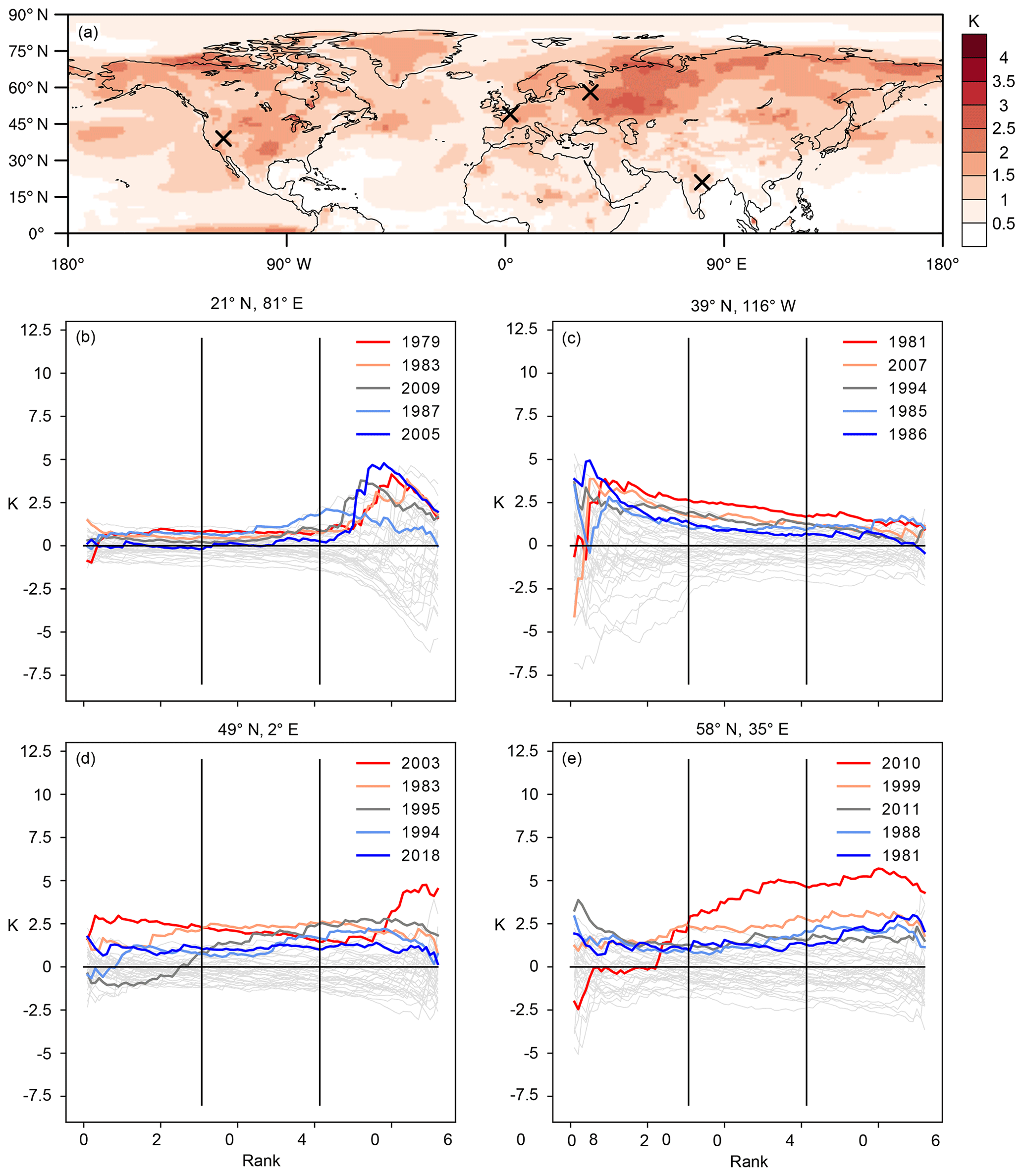
Figure 3Extreme-summer T2m anomaly and extreme-summer substructure for selected grid points in ERA-Interim. Panel (a) depicts XAERAI; panels (b)–(e) show for the five ERA-Interim extreme summers in colours and for the remaining summers in light grey. Crosses in panel (a) indicate the grid points for which the values are shown in panels (b)–(e).
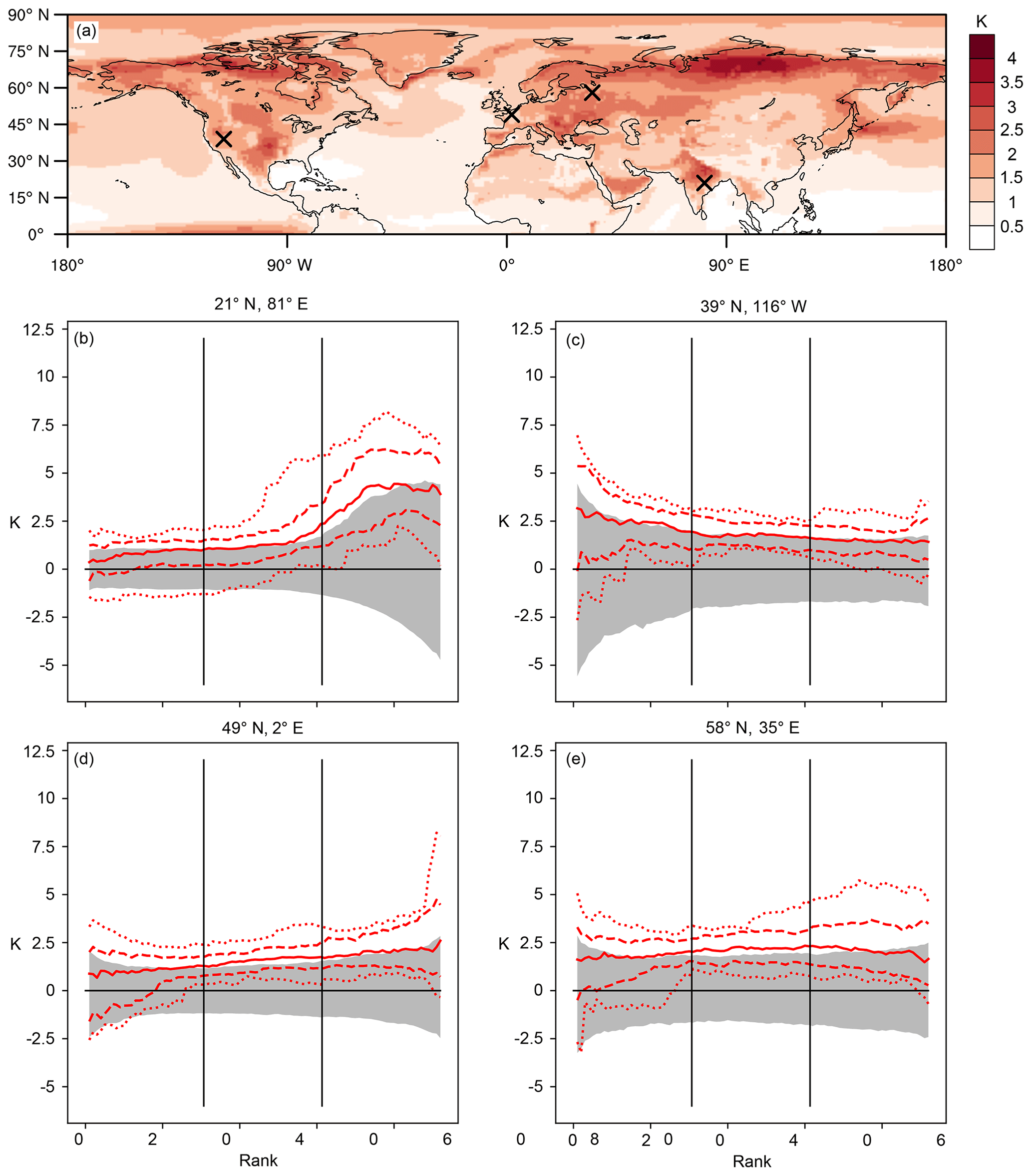
Figure 4Extreme-summer T2m anomaly and extreme-summer substructure for selected grid points in CESM. Panel (a) displays XACESM, and panels (b)–(e) show in red the maximum and minimum (dotted) 90th and 10th percentile (dashed) and the median (solid red) of the 35 CESM extreme summers. The 5th- to 95th-percentile range of the of all JJA seasons is depicted in grey. Crosses in panel (a) indicate the grid points for which the rank day anomalies are shown in panels (b)–(e).
3.2 Extreme-summer substructures at selected grid points
The rank day anomalies () for the five ERA-Interim extreme summers at a grid point located in eastern India (21∘ N, 81∘ E; Fig. 3a, b) reveal a similar substructure in at least four of the extreme summers. The largest values (up to 5 K) occur in the hottest 30 d of each season, while for the 60 coldest summer days in each extreme summer, does not exceed 1.5 K. The contributions of the coldest, middle and hottest third of all extreme-summer days to XAERAI at this grid point (i.e. , and ) are 13 %, 20 % and 67 %, respectively. For the 2005 summer, the contributions were −1 %, 6 % and 95 %, and, hence, almost the entire seasonal T2m anomaly resulted from the hottest 30 d of the summer being hotter than normal.
A comparison between the ERA-Interim and CESM extreme-summer substructures at this grid point (Figs. 3b and 4b) reveals remarkable qualitative similarities between the extreme-summer substructure at 21∘ N, 81∘ E, in the two data sets. At this grid point, also the seasons 𝕏CESM exhibit their largest values for the 30 hottest summer days. Moreover, despite the different number of seasons in the two data sets, the , and values of 11 %, 24 % and 65 %, respectively, are not far off the respective values for the seasons 𝕏ERAI. Figures 3b and 4b further reveal that the largest values reach much larger values (up to 8 K) than the values, which is an expected result, since the seasons 𝕏CESM are statistically more extreme than the seasons 𝕏ERAI.
Considering now the grid point 39∘ N, 116∘ W, in Nevada, US, we find a substantially different ERA-Interim extreme-summer substructure compared to eastern India (Fig. 3b, c), with largest extreme-summer values in the coldest third of the summer days and %, % and %. Also for this grid point, the mean substructure of CESM extreme summers is similar to that of ERA-Interim extreme summers, with %, % and % (Fig. 4c). Thus, at this grid point, all thirds of the T2m distribution contribute to extreme summers, but the contribution from the coldest third is overproportionately large (i.e. considerably larger than 33 %). Hence, the re-analysis and the climate model data both suggest that the suppression of cool summer days (leading to coldest days of the summer that are milder than usual) is a key ingredient for extreme summers at 39∘ N, 116∘ W.
A further extreme-summer substructure is apparent at the grid point closest to Paris, France (49∘ N, 2∘ E; Figs. 3d, 4d). At this grid point, the ERA-Interim extreme summer of 2018 was characterised by values of 1.5–2 K for almost all ranks; i.e. this summer resulted from an almost uniform shift in the entire T2m distribution. Moreover, this grid point also illustrates that clearly distinct extreme-summer substructures can occur at the same grid point. While the extreme summer of 2003 exhibited particularly large anomalies in the coldest and the hottest third ( %, % and %), the contribution from the coldest third to the extreme summer 1995 was negative, and the middle and top third were responsible for the entire seasonal anomaly ( %, % and %; Fig. 3d).
Finally, the grid point 58∘ N, 35∘ E, in western Russia (Fig. 3e) illustrates that, occasionally, the temperature variability during individual seasons can be fundamentally different from all other seasons at a particular grid point. Such a “regime shift” could be observed during the extreme summer of 2010, which was characterised by values in excess of 4 K for ranks ∼40–92 ( %, % and %). For these ranks, the values were almost twice as large as for the second hottest summer in these ranks (1981). The truly exceptional nature of the 2010 summer at 58∘ N, 35∘ E (e.g. Barriopedro et al. 2011; Fig. 3e), becomes even more evident when comparing its values with those of the CESM extreme summers at the same grid points (Fig. 4e). For some ranks, none of the 700 CESM JJA seasons reach values of comparable magnitude to those observed during the 2010 summer at this grid point. Some implications of this finding will be discussed in Sect. 4.
In summary, the mean extreme-summer substructure at these four grid points is qualitatively remarkably similar for the 5 hottest ERA-Interim summers and the 35 hottest CESM summers. On the one hand, this similarity implies that the rank day anomaly patterns presented in Fig. 3b–e are not artefacts of the rather short ERA-Interim period but must instead result from physical processes that shape the local extreme-summer substructure. On the other hand, these similarities suggest that the CESM is able to correctly capture the processes that generate the distinct extreme-summer substructures at these example grid points. We next compare the mean ERA-Interim and mean CESM extreme-summer substructures at all grid points in the Northern Hemisphere by considering the spatial patterns of , , and .
3.3 Spatial variability in ERA-Interim and CESM extreme-summer substructure
If extreme summers resulted from a uniform shift in the entire T2m distribution, all three thirds of the T2m distribution would contribute equally (i.e. 33 %) to XAERAI. However, the field (Fig. 5a) reveals a complex pattern of coherent regions with increased (>33 %) or decreased (<33 %) contributions from the hottest third of extreme-summer days to XAERAI. Land areas where particularly large values are found include the central US; the UK; parts of northeastern Europe, India and southeastern Asia; and the southern Sahel region (Fig. 5a). In some of these areas, exceeded and during at least four out of the five ERA-Interim extreme summers (stippling in Fig. 5a). In these regions, at least four out of the five extreme summers thus exhibited a similar substructure. However, it is important to bear in mind that in other regions the substructure of individual extreme seasons (i.e. SFcold,k, SFmiddle,k and SFhot,k) may differ from the mean extreme season substructure characterised by XFcold, XFmiddle and XFhot. Furthermore, also in parts of the northern North Pacific and northern North Atlantic, is substantially increased and reaches up to 60 %. In many regions, however, is less than 33 %, indicating that in these regions, extreme summers do not arise primarily from the hottest 30 d of the summer being hotter than they are climatologically.
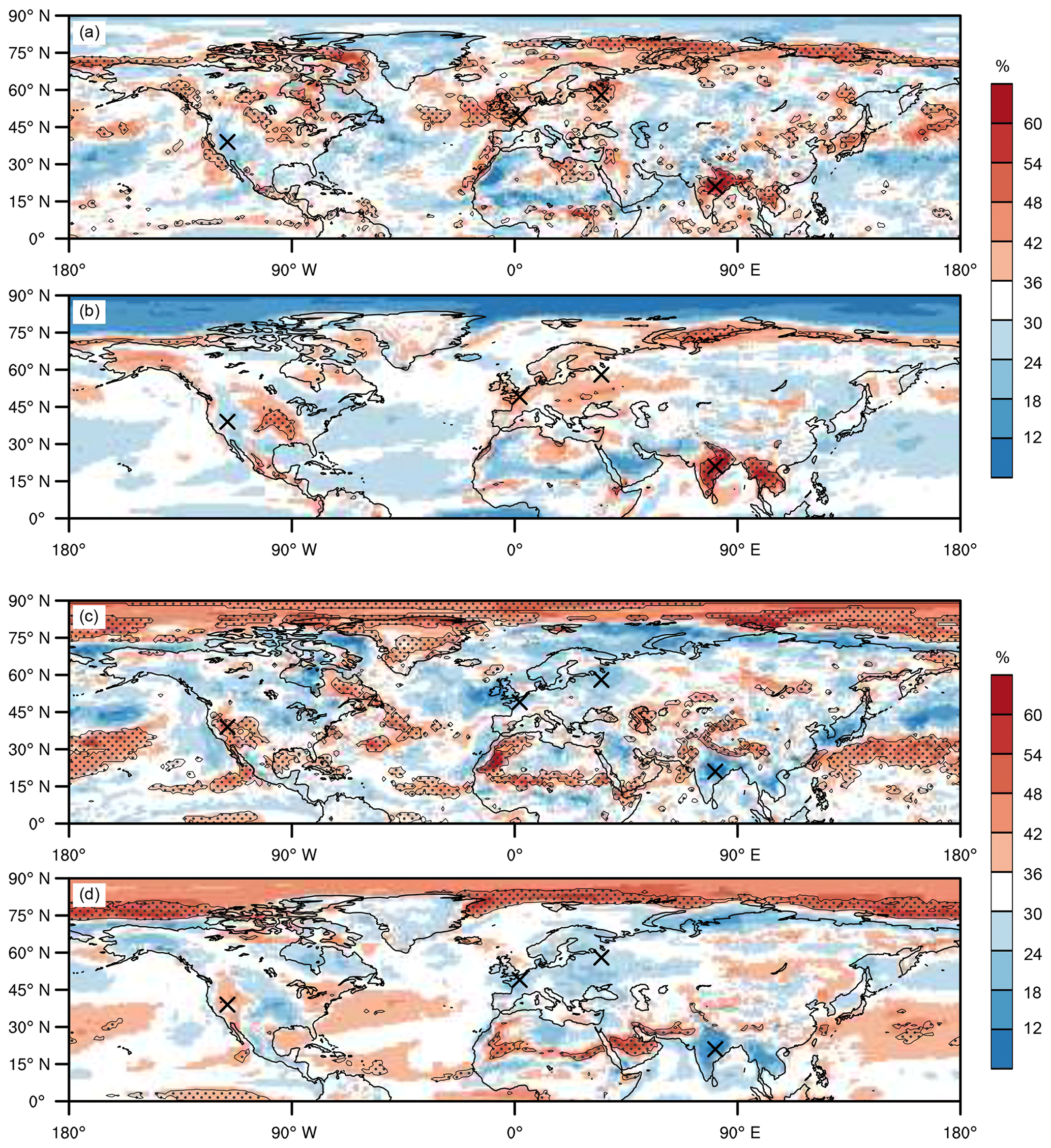
Figure 5Spatial variability in the extreme-summer substructure in ERA-Interim and CESM. Panels (a) and (b) depict and , respectively, while and are shown in panels (c) and (d). Stippled areas in all panels indicate grid points at which the same third of the distribution contributes the largest fraction of all thirds to at least 80 % of the extreme summers (i.e. similar substructure in at least 80 % of the extreme summers). Black crosses as in Fig. 3a.
In fact, in many regions it is the contribution to XAERAI from the coldest third of the summer () that is substantially increased (Fig. 5c), for example in the southwestern US, the northern Sahel region, Pakistan and parts of Greenland. Moreover, increased values are also found in the southern North Pacific and the southern North Atlantic as well as over the Arctic Ocean (Fig. 5c). Overall, Fig. 5c clearly demonstrates that the coldest third of all summer days contributes a substantial fraction to XAERAI in most regions (more than 25 % over 83 % of the Northern Hemisphere land area in ERAI). In fact, in 46 % of the Northern Hemisphere land area, exceeds ; i.e. the coldest third of extreme summers contributes more to XAERAI than the hottest third. Consequently, in these regions the mechanisms that suppress unusually cool summer days must be considered when assessing the physical causes of extremely hot summers.
Comparing these results, which are derived from ERAI with results based on CESM, i.e. and (Fig. 5a, b) as well as and (Fig. 5c, d), unravels strikingly similar patterns in many regions. For example, both data sets agree (even quantitatively) that extreme summers in India and southeastern Asia come about primarily by the hottest summer days being hotter than they are climatologically, while the coldest third of extreme-summer days only contributes a marginal fraction to the respective XA. Also in the western and central US, XFcold and XFhot agree very well between the two data sets, with the cool summer days contributing an overproportionately large fraction to XA in the western US and the hot summer days in the central US. Further areas of remarkable agreement between and (Fig. 5c, d) are the high Arctic and the northern Sahel region. Moreover, in 49 % of the Northern Hemisphere land area, exceeds , which compares well with the 46 % of the land area in which exceeds . Figure 5 thus clearly reveals that the CESM reproduces many features of the observed extreme-summer substructure and its variability in space to a remarkable degree.
However, there are also some areas of notable differences between and as well as and . For example over Greenland, Saudi Arabia and the northern North Atlantic, there are substantial differences between and (Fig. 5c, d). Moreover, over the northern North Pacific as well as the high Arctic, the and patterns agree only qualitatively but not quantitatively (Fig. 5a, b). It is important to note, though, that some differences in the XFcold and XFhot fields for the two data sets are expected due to the different sample sizes, even if the model was perfect. In the remainder of this paper we aim to explain statistical and physical reasons behind selected aspects of the spatial variability in XFcold and XFhot.
3.4 A statistical explanation for the observed extreme-summer substructures
Figures 3b and c and 4b and c clearly illustrate that, at the selected grid points in India (21∘ N, 81∘ E) and in the US (39∘ N, 116∘ W), some rank days are climatologically much more variable than others. Importantly, this is the case not just for extreme summers but is rather a climatological characteristic of the local temperature variability. For example, at 21∘ N, 81∘ E, the hottest 30 d of the summer are much more variable than the colder days. The 5th- to 95th-percentile range of the values is roughly 4 times larger than that of the values (Fig. 4b). At 39∘ N, 116∘ W, the largest rank day variability is found for lower ranks, and the 5th- to 95th-percentile range of the values is roughly 2 times smaller than the same percentile range of the values (Fig. 4c). Similar ratios are found when comparing the spread of and for these two grid points (Fig. 3b, c). Moreover, at both grid points extreme summers occur when the most variable rank days are particularly hot (Figs. 3b and c and 4b and c). Hence, from a statistical point of view, the extreme-summer substructure at these two particular grid points appears to be largely determined by the local “rank day variability pattern” – that is, the contributions to XA from the distinct rank days during extreme summers depend on how variable the respective values Td,k are climatologically.
We next assess whether the local rank day variability pattern also explains the extreme-summer substructure at other Northern Hemisphere grid points. To do so, we consider the variance (V) of the RDAd,k values of all ranks and all JJA seasons at a particular grid point:
Here we used the fact that the mean of the RDAd,k values is by construction equal to zero, and thus their variance reduces to the average of the squared RDAd,k values of all d and all k. The contribution from the coldest third of summer days to V is then
and the contributions from the middle and hottest third of the summer days to V are computed analogously.

Figure 6The variance of and its contributions from the coldest and hottest third of summer days. Panel (a) depicts VERAI, and panels (b) and (c) show and , respectively. Green contours in panels (b) and (c) depict CERAI gradient magnitudes of 6 and 12 K 10−6 m−1. The CERAI gradient magnitudes have been computed as first-order central differences and are only plotted over oceans. Black crosses as in Fig. 3a.
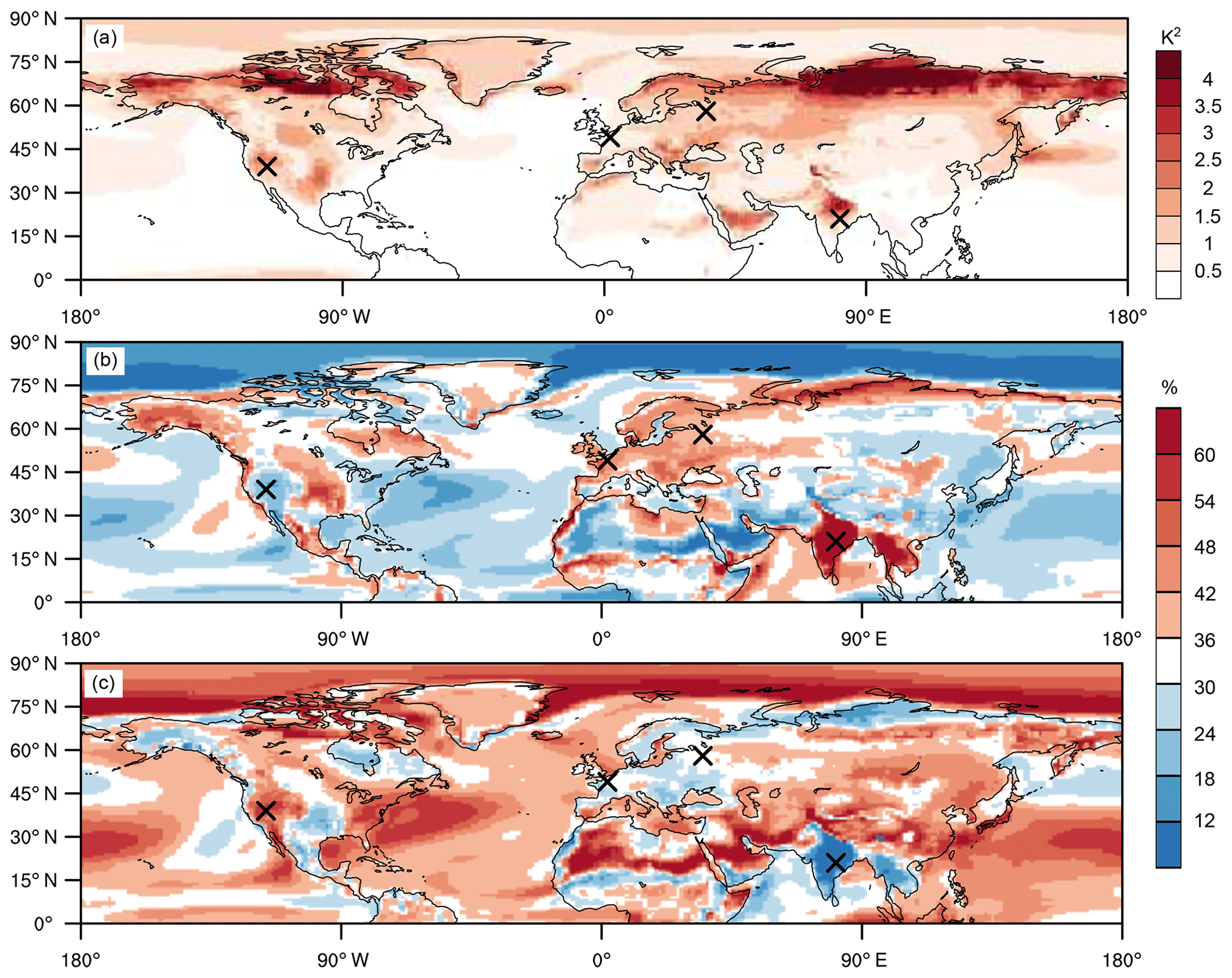
Figure 7The variance of and its contributions from the coldest and hottest third of summer days. Panel (a) depicts VCESM, and panels (b) and (c) show and , respectively. Black crosses as in Fig. 3a.
The fields of VERAI and VCESM (Figs. 6a, 7a) resemble the XAERAI and XACESM fields (Figs. 3a, 4a), as large rank day anomalies are a prerequisite for large seasonal T2m anomalies. Furthermore, comparing and (Figs. 5a and 6b) clearly reveals that wherever the contribution from the hottest third of the summer days to XAERAI is increased ( %), the rank day variability in the hottest third (quantified by ) contributes overproportionately to VERAI. Figures 5c and 6c illustrate that the same relationship also holds for and : regions where milder-than-normal cool summer days contribute overproportionately to XAERAI (i.e. %) exhibit increased values. Figures 5b and d and 7b and c confirm this finding also for the CESM data. We thus conclude that in both data sets, the extreme-summer substructure is largely determined by the local rank day variability pattern.
Furthermore, comparing the patterns of and (Figs. 6b, 7b) reveals agreement in the same regions where also the patterns of and (Fig. 5a, b) agree, and, conversely, disagreement between and also results in disagreement between and . For example, the and fields (and the and fields) are almost identical in India and southeastern Asia, the northern Sahel, the western US or eastern Europe (cf. Fig. 6b with Fig. 7b and Fig. 5a with b). Over Saudi Arabia or the northern North Atlantic, however, the patterns of and (and of and ) do not agree particularly well. In summary, while the CESM correctly reproduces the local rank day variability pattern in most regions, differences in the local rank day variability patterns between the two data sets also lead to differences in the extreme-summer substructures.
It is interesting to compare the VFcold and VFhot patterns presented in Figs. 6 and 7 with the skewness of the local daily temperature distributions, which has been studied extensively in the past (Donat and Alexander, 2012; Garfinkel and Harnik, 2017; Linz et al., 2018; Loikith et al., 2018; Loikith and Neelin, 2015; Ruff and Neelin, 2012). The upper tail of a positively skewed JJA T2m distribution, for example, is longer than the lower tail, which is the case if the hottest summer days are more variable than the coldest summer days (cf. Figs. 5b and c with Fig. S1 in the Supplement). Hence, explanations of distinct skewness in daily T2m distributions also help to understand differences in the rank day variability patterns and, subsequently, extreme-summer substructures. Garfinkel and Harnik (2017) showed that the winter low-level temperature distributions are positively skewed on the cold side of the Northern Hemisphere storm tracks, primarily because there the magnitude of warm-air advection exceeds that of cold-air advection. And, vice versa, the winter low-level temperature distributions are negatively skewed on the warm side of the Northern Hemisphere storm tracks, where the magnitude of cold-air advection exceeds that of warm-air advection. Consistent with their results, Figs. 6 and 7 depict more variable hot summer days to the north and more variable cold summer days to the south of the Northern Hemisphere storm tracks, where the horizontal gradients of T2m are particularly large (see in particular green contours in Fig. 6b, c).
While this argument explains differences in the rank day variability and the extreme-summer substructures in regions of strong surface temperature gradients, Figs. 5–7 also reveal numerous rather small-scale features that do not necessarily occur in regions of strong surface temperature gradients. We therefore next analyse the extreme-summer substructure and its causes in three example regions in more detail. Due to the similarity between the ERA-Interim and CESM extreme-summer substructures, we restrict this analysis to ERA-Interim data (except where mentioned otherwise).
3.5 (Examples of) physical causes of extreme-summer substructures
A particularly striking feature of Fig. 5 is the large contribution from the hottest third of the summer days to XAERAI in India, illustrated exemplarily for the grid point at 21∘ N, 81∘ E, in Fig. 3b. The general temperature evolution in JJA (i.e. considering all JJA seasons) at this grid point follows a particular sub-seasonal pattern (Fig. 8a). In early June, ERA-Interim T2m values are highly variable and range from 27 to almost 40∘ C, with a mean of 35∘ C on 1 June. Throughout June and the first half of July the climatological T2m drops to approximately 26∘ C and remains at this level until the end of August. Moreover, during that period, the variability in T2m is much smaller than in early June. The extreme summers exhibit comparatively high temperatures primarily in June, while in July and August their T2m evolution does not differ substantially from other JJA seasons (Fig. 8a). The drop of T2m in June is associated with the onset of the Indian summer monsoon (Fig. 8b; e.g. Slingo, 1999). During most JJA seasons, precipitation starts to fall already during the first half of June. However, the extreme summers each featured very little precipitation for at least the first 20 d of June, which suggests that extreme summers at this grid point occur when there is an unusually late onset of the Indian summer monsoon at this particular location. Moreover, the rank day variability pattern at 21∘ N, 81∘ E, is easily understood from Fig. 8: the hottest days of the season mostly occur in June and are associated with dry conditions. The onset date of the monsoon determines how many dry (and thus very hot) days occur in a JJA season; i.e. an early onset of the Indian monsoon suppresses a large number of very hot days and a late onset increases this number, which leads to the large temperature variability seen in the warmest 30 d of the JJA season.
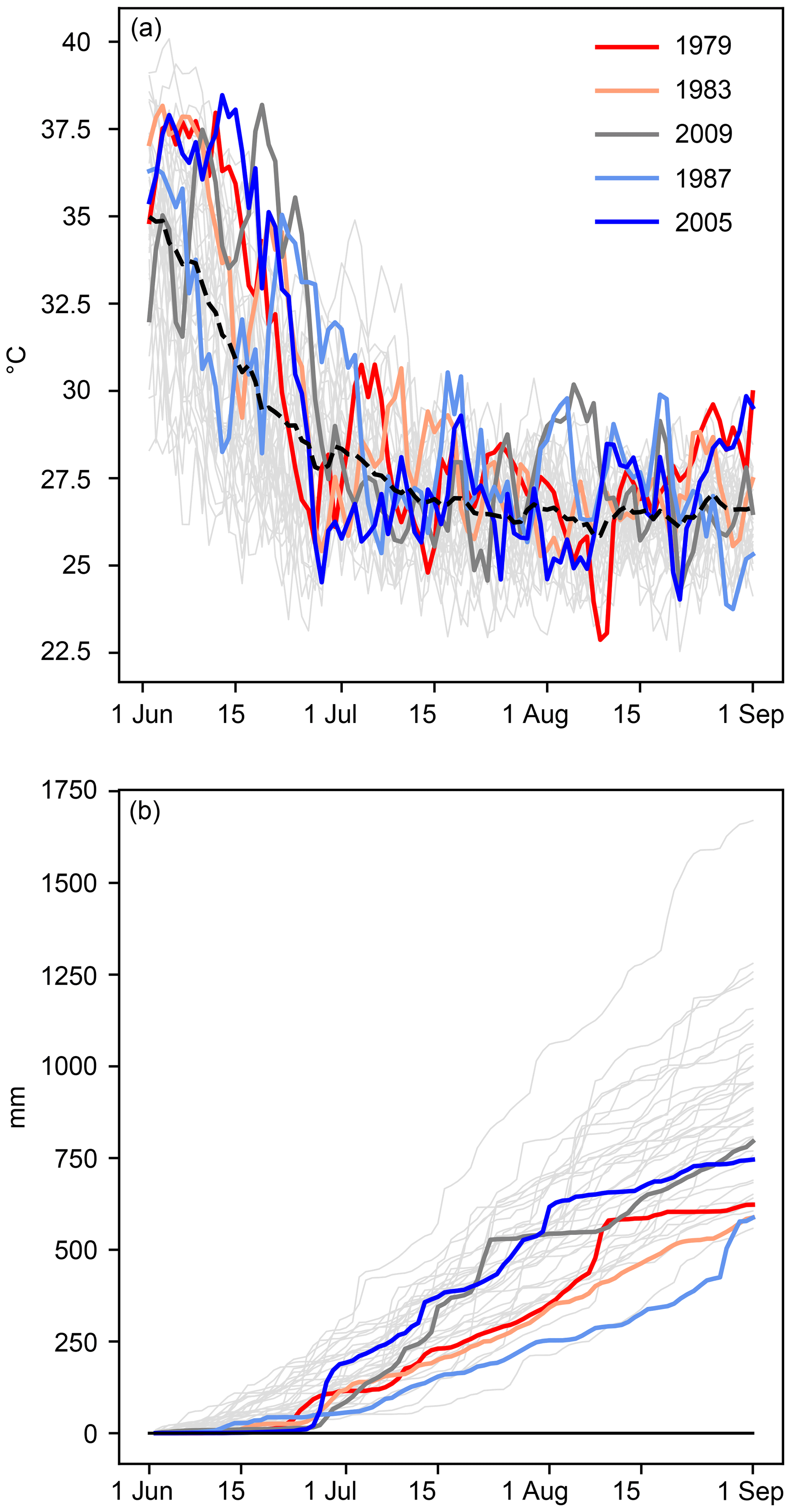
Figure 8The JJA temperature and precipitation evolution at 21∘ N, 81∘ E. Panels (a) and (b) depict non-detrended ERA-Interim T2m and accumulated precipitation at 21∘ N, 81∘ E, for all JJA seasons, respectively. The extreme summers are highlighted in colours. The dashed black line in panel (a) depicts the climatological calendar day mean T2m at 21∘ N, 81∘ E.
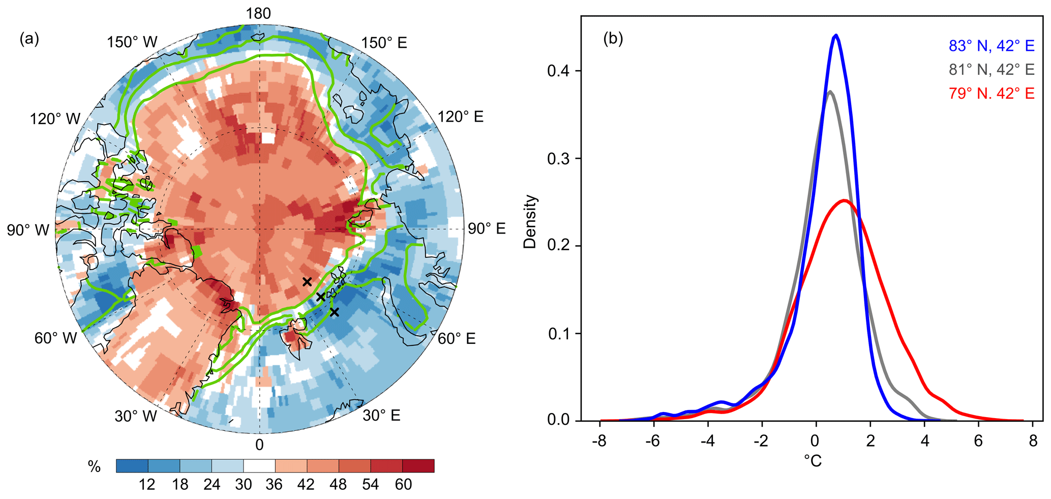
Figure 9Arctic sea ice and local summer temperature variability. (a) (shading; only 70∘ N–90∘ N is shown) and mean 1979–2018 JJA ERA-Interim sea ice concentration (green contours indicate sea ice concentrations of 0.3, 0.5 and 0.7). (b) Empirical probability density function of non-detrended ERA-Interim T2m at 79∘ N, 42∘ E (red); 81∘ N, 42∘ E (grey); and 83∘ N, 42∘ E (blue). Crosses in panel (a) locate these three grid points.
A further noteworthy feature in Fig. 5 is the sharp boundary in the extreme-summer substructure around 75–80∘ N, for example in the North Atlantic sector. North of this boundary, the coldest third of all extreme-summer days contributes up to 60 % to the extreme-summer anomaly (Fig. 5c, d). South of it, the contribution from the coldest third of extreme-summer days is much smaller. (Quantitatively, there is some disagreement between the CESM and ERAI extreme-summer substructures, but both data sets agree about the general pattern.) This sharp boundary in the extreme-summer substructure is co-located with the climatological sea ice edge in JJA (Fig. 9a). Examining the JJA T2m distributions at three grid points across this boundary (83∘ N, 42∘ W; 81∘ N, 42∘ W; and 79∘ N, 42∘ W) reveals that for T2m below −1∘ C, their probability density functions (pdf's) of the daily T2m values are almost identical, which is not surprising due to their close spatial proximity. However, large differences in the three pdf's are found for T2m at about 0∘ C and above. At 83∘ N, i.e. north of the climatological sea ice edge (Fig. 9a), the pdf exhibits a very short upper tail with very little probability density exceeding +2∘ C (i.e. the pdf is strongly negatively skewed), while at 79∘ N (i.e. south of the climatological sea ice edge) the upper tail is much more variable. The geographical co-location of this extreme-summer substructure boundary and of the climatological sea ice edge is striking and suggests that the contrasting substructures arise because the sea ice buffers “warm” temperatures at 0∘ C – that is, air with T2m >0∘ C is cooled down to close to 0∘ C by the induced sea ice melting. The same effect has also been shown to shorten the upper tail of the surface temperature pdf over snow-covered areas (Loikith et al., 2018).
As a third example, we return to the grid point in Nevada, US (at 39∘ N, 116∘ W), where the rank day variability is largest for the cold summer days and extreme summers occur when the coldest 30 d exhibit mostly large positive rank day anomalies (Figs. 3c and 4c). Thus, at this grid point, milder-than-normal coldest days of the summer (or, equivalently, suppressed cool summer days) are a key ingredient for extreme summers. We therefore briefly explore why, at this grid point, the coldest summer days during extreme summers are warmer than normal.
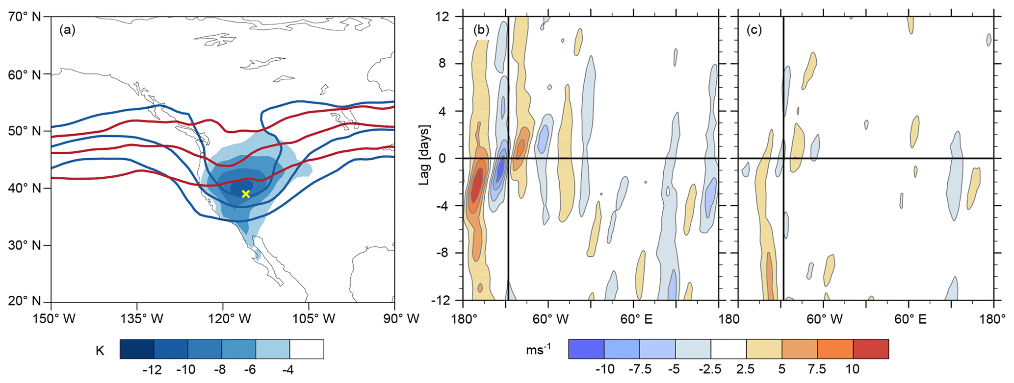
Figure 10(a) T2m difference between the 100 climatologically coldest JJA days and the 100 coldest extreme-summer days (shading). Contours depict the composite PV field at 335 K (contours of 2, 3.5 and 5 PVU) for the 100 climatologically coldest JJA days (blue) and for the 100 coldest extreme-summer days (red). The yellow cross indicates 39∘ N, 116∘ W. Panels (b) and (c) depict composite Hovmöller diagrams of the anomalous 250 hPa meridional wind, averaged between 35 and 65∘ N, and temporally centred on the 100 climatologically coldest JJA days (b) and on the 100 coldest extreme-summer days (c). Meridional wind anomalies are calculated relative to the 1979–2018 mean JJA meridional wind. The vertical line in panel (b) and (c) indicates 116∘ W.
We first investigate what makes the climatologically coldest summer days at 39∘ N, 116∘ W, particularly cold and then contrast them with the coldest summer days during extreme summers at 39∘ N, 116∘ W. A composite analysis of the upper-level flow during the 100 climatologically coldest ERA-Interim days of all 1979–2018 summers unravels a characteristic upper-level flow pattern: a highly amplified Rossby wave pattern over the eastern North Pacific and North America, with a breaking synoptic-scale trough covering 39∘ N, 116∘ W (Fig. 10a). The breaking Rossby wave causing the trough is part of a synoptic-scale and transient wave packet (Fig. 10b) which has just the right phasing such that the trough axis crosses 39∘ N, 116∘ W, when the amplitude of the trough is largest (Fig. 10b). This type of relatively small-scale trough, shown here with contours of potential vorticity on an isentrope in the upper troposphere (Fig. 10a), is relatively slow-moving (Fig. 10b), such that the induced northwesterly low-level flow along its western flank can lead to strong and persistent cold-air advection to the western US. Additionally, the low-level flow induced by the trough impinges on the topography at the US West Coast. Consequently, low-level air masses that are advected into the western US are most likely forced to ascend, which leads to adiabatic cooling of these already cool air masses and finally results in the climatologically coldest summer days at 39∘ N, 116∘ W.
The composites for the 100 coldest days during extreme summers, in contrast, do not reveal such a wave pattern (Fig. 10a and c). This indicates that the flow pattern characteristic of the climatologically coldest days at this grid point, i.e. the Rossby wave breaking and trough formation with the phasing discussed above, simply did not occur very often during extreme summers. Furthermore, a synoptic analysis of these 100 coldest extreme-summer days (not shown) reveals that the associated upper-level flow configurations are rather variable, some featuring troughs while others even exhibited low-amplitude ridges, resulting in the rather zonal composite upper-level flow apparent in Fig. 10a and c.
The reason why such highly amplified troughs with the right phasing did not occur during extreme summers at 39∘ N, 116∘ W, is currently unclear and at the same time challenging to assess. Possibly, the exact longitude where the synoptic-scale waves have been triggered (Röthlisberger et al., 2018) as well as the strength and longitudinal extent of the North Pacific jet, which modulates the waves' downstream propagation and breaking behaviour (e.g. Drouard et al. 2015), might have played a role. However, both the jet strength and the characteristics of the transient waves propagating along the jet are strongly modulated by lower-frequency processes such as the Madden–Julian Oscillation (Moore et al., 2010) and the El Niño–Southern Oscillation (Drouard et al., 2015; Shapiro et al., 2001). This example thus illustrates that a seamless approach, combining processes on different timescales, is most likely required to fully reveal the physical causes of extreme summers.
In this study, extreme summers are defined in the upper tail of the JJA seasonal mean T2m distribution at each grid point in the Northern Hemisphere and then analysed with regard to their substructure. Hereby, the extreme-summer T2m anomaly is decomposed into its contribution from each rank day. First, all days are ranked within their respective season (i.e. from rank 1 to 92 for JJA) and then compared to the climatological T2m of all days with the same rank. The resulting rank day anomalies exactly quantify how much each (rank) day contributes to the T2m anomaly of the respective season and therefore allow for very intuitive statements about the characteristics of extreme summers. For example, we show that during the 2010 summer at the ERAI grid point at 58∘ N, 35∘ E, the 31 hottest days contributed 53 % to the seasonal anomaly of 3.13 K and were each at least 4 K warmer than they are climatologically. This decomposition is applied to T2m data from ERA-Interim as well as data from 700 simulated years with CESM for present-day climate conditions. Thereby, the contributions from the coldest, middle and hottest third of extreme summers to the extreme-summer T2m anomalies are quantified at each Northern Hemisphere grid point (XFcold, XFmiddle and XFhot).
This analysis reveals clearly distinct extreme-summer substructures, occurring in coherent geographical regions. Despite the relatively small scale of the structures in the and fields as well as different numbers of extreme summers in the two data sets, CESM is able to reproduce these fields to a remarkable degree. This result firstly underlines that the ERA-Interim extreme-summer substructures and their spatial variability result from physical processes rather than too short a data record and, secondly, testifies to the model's ability to reproduce the physical processes responsible for the occurrence of extreme summers in most regions in the Northern Hemisphere. Areas where CESM and ERA-Interim extreme-summer substructures differ include Greenland, the northern North Atlantic and the Arabian Peninsula.
Furthermore, a key finding of this study is that the mean extreme-summer substructure is consistent with the shape of the underlying local T2m distribution. The extreme-summer substructure is largely determined by which of the 92 JJA rank days are most variable (i.e. the rank day variability pattern), which is qualitatively related to the skewness of the T2m distribution. Simply speaking, in regions where the coldest days of the summer are most variable (i.e. negatively skewed T2m distribution), extreme summers occur when the coldest days of the summer are unusually hot and, analogously, for the case where hottest days vary the most (i.e. positively skewed T2m distribution). This finding is relevant for two reasons. Firstly, it constrains what kind of extreme-summer substructures can locally be expected, in particular in regions with strongly skewed daily temperature distributions. For example, extreme summers arising primarily from extremely hot summer days (i.e. heat waves) are unlikely to occur in regions with strongly negatively skewed temperature distributions. Secondly, some individual extreme summers such as the 2010 summer at the grid point at 58∘ N, 35∘ E, featured clear temperature regime shifts, with rank day anomalies far outside of what could be expected from their climatological variability (e.g. almost twice as large as the second large anomalies for the same ranks during the 2010 summer at 58∘ N, 35∘ E). The general consistency between the mean extreme-summer substructure and the skewness of the underlying T2m distribution illustrates that such regime shifts in the temperature variability during extreme summers are the exception rather than the norm.
This consistency furthermore allows us to rely on previous work on physical causes of skewed surface temperature distributions for interpreting our results. Consistent with the findings of Garfinkel and Harnik (2017), we find distinct extreme-summer substructures relative to the location of large surface temperature gradients, in particular in the Northern Hemisphere storm track regions. Extreme summers occurring north of the Northern Hemisphere storm tracks have large contributions from the hottest third of summer days, and south of the storm tracks the contributions from the coldest days are largest. This is primarily because on the cold side of a temperature gradient, warm-air advection can reach much larger magnitudes than cold-air advection, and vice versa on the warm side (e.g. Garfinkel and Harnik, 2017; Linz et al., 2018; Tamarin-Brodsky et al., 2019). Moreover, the few areas where the ERA-Interim and CESM extreme-summer substructures differ also have distinct rank day variability patterns in ERA-Interim and CESM. Thus, the climate model's ability to reproduce the ERA-Interim extreme-summer substructures in most places results largely from the model's ability to produce local rank day variability patterns that agree with ERA-Interim.
However, three case studies illustrate that the extreme-summer substructure cannot always be explained by temperature advection alone. In eastern India, more than 65 % of the extreme-summer T2m anomaly results from the hottest 30 d of JJA being hotter than they are climatologically. At the considered grid point, T2m exhibits a distinct sub-seasonal pattern, as it typically drops by almost 10 K with the onset of the Indian summer monsoon. Thus, the hottest days of the season (occurring in June) are highly variable, and extreme summers occur in seasons with particularly late monsoon onsets.
In the high Arctic the highest surface temperatures are buffered around 0∘ C, as excess heat would result in sea ice melting and subsequent latent cooling. Hence, the cold part of the T2m distribution accounts for most of the rank day anomaly variance, and, consequently, extreme summers occur when the coldest summer days are warmer than normal. This buffering effect of the Arctic sea ice leads to a strong boundary in the extreme-summer substructure around 75–80∘ N, i.e. near the climatological JJA sea ice edge.
At a grid point in the western United States, all parts of the T2m distribution contribute significantly to extreme summers; however, an overproportionately large fraction comes from the coldest third of the extreme-summer days (i.e. the coldest extreme-summer days are warmer than their rank day mean). Composites of the upper-level flow during the 100 climatologically coldest summer days reveal that an amplified upper-level flow pattern with a particular phasing of a prominent trough and its associated cold-air advection is characteristic of the climatologically coldest summer days at this grid point. This particular flow pattern did not occur frequently during the extreme summers, leading to milder-than-normal cool summer days. This result is consistent with previous work on physical causes of non-Gaussian temperature distributions (Garfinkel and Harnik, 2017; Linz et al., 2018; Tamarin-Brodsky et al., 2019), as it highlights the role of temperature advection by transient waves in generating a non-uniform rank day variability pattern, or similarly, a skewed T2m distribution.
Overall, the case studies illustrate that for understanding the physical causes of extreme summers, a seamless approach is necessary, which combines weather system dynamics, local thermodynamics and surface–atmosphere interactions as well as lower frequency variability in the atmosphere and the ocean. Clearly, distinct physical causes might lead to similar extreme-summer substructures, in particular when comparing regions that are far apart (e.g. the northern Sahel region and the high Arctic; Fig. 5). However, similar extreme-summer substructures in neighbouring regions conceivably also point to similar physical causes of extreme summers (e.g. the Asian Monsoon region). Therefore, the extreme-summer substructure is a helpful tool for discriminating between neighbouring regions with distinct physical causes of extreme summers and might also be helpful for identifying coherent regions with similar physical causes of extreme summers.
A further key result of this study is that in most places, the cool summer days contribute substantially to extreme-summer T2m anomalies (more than 25 % over 83 % of the Northern Hemisphere land area in ERAI). In fact, Fig. 5 reveals that for ERA-Interim (CESM) in 46 % (49 %) of the Northern Hemisphere land area, the coldest third of the summer contributes more to the extreme-summer anomaly (XA) than the hottest third. Thus, large positive seasonal temperature anomalies (i.e. extreme summers as opposed to individual heat waves) cannot be understood and explained by only considering the physical drivers of heat waves. Rather, the processes which suppress the occurrence of cold summer days must also be considered. These processes, though, are so far virtually unexplored and thus possibly yield an untapped potential for improving our understanding of extreme summers. However, as illustrated by the example of extreme summers in the western US, the processes that suppress the occurrence of cold summer days sometimes seem rather intangible, as they do not necessarily manifest themselves in the occurrence of an unusual flow pattern but rather in the non-occurrence of the particular flow pattern that typically produces the coldest summer days.
This study has illustrated that extreme summers across the Northern Hemisphere have distinct substructures, which result directly from the physical causes of the extreme summers. However, the concept of the extreme season substructure has applications beyond what has been presented in this study and thus calls for subsequent studies. Firstly, the presented analyses could be extended to the Southern Hemisphere and other seasons and variables. (The application of the technique is most promising for variables that are potentially unbound and variable on both ends, i.e. not for a positive definite variable like precipitation.) Secondly, the concept of a “season substructure” can be relevant for field campaigns, as the representativeness of the campaigns' measurements depends on how representative the time period of the campaign was (Wernli et al., 2010). Thirdly, extreme summers with distinct substructures conceivably have different societal effects, and thus future research should assess whether or not and where the extreme-summer substructure is affected by climate change. The results of this study suggest that the CESM is a suitable tool for this task, as it is largely able to reproduce the observed (ERA-Interim) extreme-summer substructure in the current climate. However, some of the extreme summers observed within the last 40 years appear to be outside of the spectrum of 700 years of CESM. Hence, while CESM is able to reproduce the local extreme-summer substructures, it may not be able to reproduce the most extreme summers that are physically possible in some regions. Clearly, this finding requires detailed and critical further investigation. Finally, changes in the extreme-summer substructure with climate change must be related to changes in the physical causes of extreme summers, as a uniform warming would not affect the local rank day variability pattern. Therefore, contrasting extreme-summer substructures in present and future climate simulations might also help to identify regions where the physical causes of extreme summers are altered by climate change.
ERA-Interim data can be downloaded from the ECMWF web page at: https://apps.ecmwf.int/datasets/data/interim-full-daily/levtype=sfc/ (European Centre for Medium-Range Weather Forecasts, 2020). The CESM T2m data used here are available upon request from the authors.
The supplement related to this article is available online at: https://doi.org/10.5194/wcd-1-45-2020-supplement.
MR and HW conceived the study, MS provided technical support, UB performed the CESM simulations, and MR analysed the data and wrote the major part of the paper. HW, EF, MS and UB also contributed to writing the paper and commented on earlier versions of this paper.
The authors declare that they have no conflict of interest.
Maxi Boettcher (ETH Zürich) and Lukas Papritz (ETH Zürich) are acknowledged for helpful discussions during different stages of this work; Gary Strand (NCAR) and Clara Deser (NCAR) are acknowledged for providing the CESM restart files; and two anonymous reviewers are acknowledged for providing thoughtful, challenging yet encouraging reviews.
This research has been supported by the H2020 European Research Council (INTEXseas (grant no. 787652)).
This paper was edited by Peter Knippertz and reviewed by two anonymous referees.
Barriopedro, D., Fischer, E., Luterbacher, J., Trigo, R., and Ricardo, G.-H.: The hot summer of 2010: Redrawing the temperature record map of Europe, Test, 332, 220–224, https://doi.org/10.1126/science.1201224, 2011.
Brunner, L., Hegerl, G. C., and Steiner, A. K.: Connecting atmospheric blocking to European temperature extremes in spring, J. Climate, 30, 585–594, https://doi.org/10.1175/JCLI-D-16-0518.1, 2017.
Buras, A., Rammig, A., and Zang, C. S.: Quantifying impacts of the drought 2018 on European ecosystems in comparison to 2003, Biogeosciences Discuss., https://doi.org/10.5194/bg-2019-286, in review, 2019.
Ciais, P., Reichstein, M., Viovy, N., Granier, A., Ogée, J., Allard, V., Aubinet, M., Buchmann, N., Bernhofer, C., Carrara, A., Chevallier, F., De Noblet, N., Friend, A. D., Friedlingstein, P., Grünwald, T., Heinesch, B., Keronen, P., Knohl, A., Krinner, G., Loustau, D., Manca, G., Matteucci, G., Miglietta, F., Ourcival, J. M., Papale, D., Pilegaard, K., Rambal, S., Seufert, G., Soussana, J. F., Sanz, M. J., Schulze, E. D., Vesala, T., and Valentini, R.: Europe-wide reduction in primary productivity caused by the heat and drought in 2003, Nature, 437, 529–533, https://doi.org/10.1038/nature03972, 2005.
Cohen, J., Screen, J. A., Furtado, J. C., Barlow, M., Whittleston, D., Coumou, D., Francis, J., Dethloff, K., Entekhabi, D., Overland, J., and Jones, J.: Recent Arctic amplification and extreme mid-latitude weather, Nat. Geosci., 7, 627–637, https://doi.org/10.1038/ngeo2234, 2014.
Dee, D. P., Uppala, S. M., Simmons, A. J., Berrisford, P., Poli, P., Kobayashi, S., Andrae, U., Balmaseda, M. A., Balsamo, G., Bauer, P., Bechtold, P., Beljaars, A. C. M., van de Berg, L., Bidlot, J., Bormann, N., Delsol, C., Dragani, R., Fuentes, M., Geer, A. J., Haimberger, L., Healy, S. B., Hersbach, H., Hólm, E. V., Isaksen, L., Kållberg, P., Köhler, M., Matricardi, M., Mcnally, A. P., Monge-Sanz, B. M., Morcrette, J.-J., Park, B.-K., Peubey, C., de Rosnay, P., Tavolato, C., Thépaut, J. N., and Vitart, F.: The ERA-Interim reanalysis: Configuration and performance of the data assimilation system, Q. J. Roy. Meteor. Soc., 137, 553–597, https://doi.org/10.1002/qj.828, 2011.
Donat, M. G. and Alexander, L. V.: The shifting probability distribution of global daytime and night-time temperatures, Geophys. Res. Lett., 39, L14707, https://doi.org/10.1029/2012GL052459, 2012.
Dong, B., Sutton, R., Shaffrey, L., and Wilcox, L.: The 2015 European heat wave, B. Am. Meteorol. Soc., 97, 57–62, https://doi.org/10.1175/BAMS-D-16-0140.1, 2016.
Drouard, M., Rivière, G., and Arbogast, P.: The link between the North Pacific climate variability and the North Atlantic Oscillation via downstream propagation of synoptic waves, J. Climate, 28, 3957–3976, https://doi.org/10.1175/JCLI-D-14-00552.1, 2015.
European Centre for Medium-Range Weather Forecasts: ERA-Interim re-analysis data, available at: https://apps.ecmwf.int/datasets/data/interim-full-daily/levtype=sfc/, last access: 21 February 2020.
Fink, A. H., Brücher, T., Krüger, A., Leckebusch, G. C., Pinto, J. G., and Ulbrich, U.: The 2003 European summer heatwaves and drought – synoptic diagnosis and impacts, Weather, 59, 209–216, https://doi.org/10.1256/wea.73.04, 2004.
Fischer, E. M., Seneviratne, S. I., Vidale, P. L., Lüthi, D., and Schär, C.: Soil moisture-atmosphere interactions during the 2003 European summer heat wave, J. Climate, 20, 5081–5099, https://doi.org/10.1175/JCLI4288.1, 2007.
Fischer, E. M., Beyerle, U., and Knutti, R.: Robust spatially aggregated projections of climate extremes, Nat. Clim. Chang., 3, 1033–1038, https://doi.org/10.1038/nclimate2051, 2013.
Fouillet, A., Rey, G., Laurent, F., Pavillon, G., Bellec, S., Guihenneuc-Jouyaux, C., Clavel, J., Jougla, E., and Hémon, D.: Excess mortality related to the August 2003 heat wave in France, Int. Arch. Occup. Environ. Health, 80, 16–24, https://doi.org/10.1007/s00420-006-0089-4, 2006.
Garfinkel, C. I. and Harnik, N.: The non-Gaussianity and spatial asymmetry of temperature extremes relative to the storm track: The role of horizontal advection, J. Climate, 30, 445–464, https://doi.org/10.1175/JCLI-D-15-0806.1, 2017.
Hoskins, B.: The potential for skill across the range of the seamless weather-climate prediction problem: A stimulus for our science, Q. J. Roy. Meteor. Soc., 139, 573–584, https://doi.org/10.1002/qj.1991, 2013.
Hoy, A., Hänsel, S., Skalak, P., Ustrnul, Z., and Bochníček, O.: The extreme European summer of 2015 in a long-term perspective, Int. J. Climatol., 37, 943–962, https://doi.org/10.1002/joc.4751, 2017.
Hurrell, J. W., Holland, M. M., Gent, P. R., Ghan, S., Kay, J. E., Kushner, P. J., Lamarque, J.-F., Large, W. G., Lawrence, D., Lindsay, K., Lipscomb, W. H., Long, M. C., Mahowald, N., Marsh, D. R., Neale, R. B., Rasch, P., Vavrus, S., Vertenstein, M., Bader, D., Collins, W. D., Hack, J. J., Kiehl, J., Marshall, S., Hurrell, J. W., Holland, M. M., Gent, P. R., Ghan, S., Kay, J. E., Kushner, P. J., Lamarque, J.-F., Large, W. G., Lawrence, D., Lindsay, K., Lipscomb, W. H., Long, M. C., Mahowald, N., Marsh, D. R., Neale, R. B., Rasch, P., Vavrus, S., Vertenstein, M., Bader, D., Collins, W. D., Hack, J. J., Kiehl, J., and Marshall, S.: The Community Earth System Model: A framework for collaborative research, B. Am. Meteorol. Soc., 94, 1339–1360, https://doi.org/10.1175/BAMS-D-12-00121.1, 2013.
Kay, J. E., Deser, C., Phillips, A., Mai, A., Hannay, C., Strand, G., Arblaster, J. M., Bates, S. C., Danabasoglu, G., Edwards, J., Holland, M., Kushner, P., Lamarque, J.-F., Lawrence, D., Lindsay, K., Middleton, A., Munoz, E., Neale, R., Oleson, K., Polvani, L., Vertenstein, M., Kay, J. E., Deser, C., Phillips, A., Mai, A., Hannay, C., Strand, G., Arblaster, J. M., Bates, S. C., Danabasoglu, G., Edwards, J., Holland, M., Kushner, P., Lamarque, J.-F., Lawrence, D., Lindsay, K., Middleton, A., Munoz, E., Neale, R., Oleson, K., Polvani, L., and Vertenstein, M.: The Community Earth System Model (CESM) Large Ensemble Project: A community resource for studying climate change in the presence of internal climate variability, B. Am. Meteorol. Soc., 96, 1333–1349, https://doi.org/10.1175/BAMS-D-13-00255.1, 2015.
Linz, M., Chen, G., and Hu, Z.: Large-scale atmospheric control on non-Gaussian tails of midlatitude temperature distributions, Geophys. Res. Lett., 45, 9141–9149, https://doi.org/10.1029/2018GL079324, 2018.
Loikith, P. C. and Neelin, J. D.: Short-tailed temperature distributions over North America and implications for future changes in extremes, Geophys. Res. Lett., 42, 8577–8585, https://doi.org/10.1002/2015GL065602, 2015.
Loikith, P. C., Neelin, J. D., Meyerson, J., and Hunter, J. S.: Short warm-side temperature distribution tails drive hot spots of warm temperature extreme increases under near-future warming, J. Climate, 31, 9469–9487, https://doi.org/10.1175/JCLI-D-17-0878.1, 2018.
Lorenz, R., Jaeger, E. B., and Seneviratne, S. I.: Persistence of heat waves and its link to soil moisture memory, Geophys. Res. Lett., 37, L09703, https://doi.org/10.1029/2010GL042764, 2010.
Moore, R. W., Martius, O., and Spengler, T.: The modulation of the subtropical and extratropical atmosphere in the Pacific basin in response to the Madden–Julian oscillation, Mon. Weather Rev., 138, 2761–2779, https://doi.org/10.1175/2010MWR3194.1, 2010.
Orth, R., Zscheischler, J., and Seneviratne, S. I.: Record dry summer in 2015 challenges precipitation projections in Central Europe, Sci. Rep., 6, 28334, https://doi.org/10.1038/srep28334, 2016.
Pfahl, S. and Wernli, H.: Quantifying the relevance of atmospheric blocking for co-located temperature extremes in the Northern Hemisphere on (sub-)daily time scales, Geophys. Res. Lett., 39, 1–6, https://doi.org/10.1029/2012GL052261, 2012.
Röthlisberger, M. and Martius, O.: Quantifying the local effect of Northern Hemisphere atmospheric blocks on the persistence of summer hot and dry spells, Geophys. Res. Lett., 46, 10101–10111, https://doi.org/10.1029/2019GL083745, 2019.
Röthlisberger, M., Martius, O., and Wernli, H.: Northern Hemisphere Rossby wave initiation events on the extratropical jet–A climatological analysis, J. Climate, 31, 743–760, https://doi.org/10.1175/JCLI-D-17-0346.1, 2018.
Röthlisberger, M., Frossard, L., Bosart, L. F., Keyser, D., and Martius, O.: Recurrent synoptic-scale Rossby wave patterns and their effect on the persistence of cold and hot spells, J. Climate, 32, 3207–3226, https://doi.org/10.1175/JCLI-D-18-0664.1, 2019.
Ruff, T. W. and Neelin, J. D.: Long tails in regional surface temperature probability distributions with implications for extremes under global warming, Geophys. Res. Lett., 39, L04704, https://doi.org/10.1029/2011GL050610, 2012.
Russo, S., Sillmann, J., and Fischer, E. M.: Top ten European heatwaves since 1950 and their occurrence in the coming decades, Environ. Res. Lett., 10, 124003, https://doi.org/10.1088/1748-9326/10/12/124003, 2015.
Schär, C. and Jendritzky, G.: Hot news from summer 2003, Nature, 432, 559–560, https://doi.org/10.1038/432559a, 2004.
Schneidereit, A., Schubert, S., Vargin, P., Lunkeit, F., Zhu, X., Peters, D. H. W., and Fraedrich, K.: Large-scale flow and the long-lasting blocking high over Russia: Summer 2010, Mon. Weather Rev., 140, 2967–2981, https://doi.org/10.1175/MWR-D-11-00249.1, 2012.
Seneviratne, S. I., Corti, T., Davin, E. L., Hirschi, M., Jaeger, E. B., Lehner, I., Orlowsky, B., and Teuling, A. J.: Investigating soil moisture-climate interactions in a changing climate: A review, Earth-Sci. Rev., 99, 125–161, https://doi.org/10.1016/j.earscirev.2010.02.004, 2010.
Shapiro, M. A., Wernli, H., Bond, N. A., and Langland, R.: The influence of the 1997–99 El Niňo Southern Oscillation on extratropical baroclinic life cycles over the eastern North Pacific, Q. J. Roy. Meteor. Soc., 127, 331–342, https://doi.org/10.1002/qj.49712757205, 2001.
Slingo, J.: The Indian summer monsoon and its variability, in: Beyond El Niño: Decadal and interdecadal climate variability, edited by: Navarra, A., Springer, Berlin, Germany, 103–116, 1999.
Sousa, P. M., Trigo, R. M., Barriopedro, D., Soares, P. M. M., and Santos, J. A.: European temperature responses to blocking and ridge regional patterns, Clim. Dyn., 50, 457–477, https://doi.org/10.1007/s00382-017-3620-2, 2018.
Tamarin-Brodsky, T., Hodges, K., Hoskins, B. J., and Shepherd, T. G.: A dynamical perspective on atmospheric temperature variability and its response to climate change, J. Climate, 32, 1707–1724, https://doi.org/10.1175/JCLI-D-18-0462.1, 2019.
Vogel, M. M., Zscheischler, J., Wartenburger, R., Dee, D., and Seneviratne, S. I.: Concurrent 2018 hot extremes across Northern Hemisphere due to human-induced climate change, Earth's Future, 7, 2019EF001189, https://doi.org/10.1029/2019EF001189, 2019.
Wehner, M., Stone, D., Krishnan, H., AchutaRao, K., and Castillo, F.: The deadly combination of heat and humidity in India and Pakistan in summer 2015, B. Am. Meteorol. Soc., 97, 81–86, https://doi.org/10.1175/BAMS-D-16-0145.1, 2016.
Wernli, H., Pfahl, S., Trentmann, J., and Zimmer, M.: How representative were the meteorological conditions during the COPS field experiment in summer 2007?, Meteorol. Z., 19, 619–630, https://doi.org/10.1127/0941-2948/2010/0483, 2010.
Zschenderlein, P., Fink, A. H., Pfahl, S., and Wernli, H.: Processes determining heat waves across different European climates, Q. J. Roy. Meteor. Soc., 145, 2973–2989, https://doi.org/10.1002/qj.3599, 2019.
The requested paper has a corresponding corrigendum published. Please read the corrigendum first before downloading the article.
- Article
(14066 KB) - Full-text XML
- Corrigendum
-
Supplement
(377 KB) - BibTeX
- EndNote
extreme-summer substructurevaries substantially across the Northern Hemisphere and is directly related to the local physical drivers of extreme summers. Furthermore, comparing re-analysis (i.e. measurement-based) and climate model extreme-summer substructures reveals a remarkable level of agreement.