the Creative Commons Attribution 4.0 License.
the Creative Commons Attribution 4.0 License.
 | 04 Feb 2020
Extratropical-cyclone-induced sea surface temperature anomalies in the 2013–2014 winter
Helen F. Dacre
Simon A. Josey
Alan L. M. Grant
The 2013–2014 winter averaged sea surface temperature (SST) was anomalously cool in the mid-North Atlantic region. This season was also unusually stormy, with extratropical cyclones passing over the mid-North Atlantic every 3 d. However, the processes by which cyclones contribute towards seasonal SST anomalies are not fully quantified. In this paper a cyclone identification and tracking method is combined with European Centre for Medium-Range Weather Forecasts (ECMWF) atmosphere and ocean reanalysis fields to calculate cyclone-relative net surface heat flux anomalies and resulting SST changes. Anomalously large negative heat flux is located behind the cyclones' cold front, resulting in anomalous cooling up to 0.2 K d−1 when the cyclones are at maximum intensity. This extratropical-cyclone-induced “cold wake” extends along the cyclones' cold front but is small compared to climatological variability in the SSTs. To investigate the potential cumulative effect of the passage of multiple cyclone-induced SST cooling in the same location, we calculate Earth-relative net surface heat flux anomalies and resulting SST changes for the 2013–2014 winter period. Anomalously large winter averaged negative heat flux occurs in a zonally orientated band extending across the North Atlantic between 40 and 60∘ N. The 2013–2014 winter SST cooling anomaly associated with air–sea interactions (ASIs; anomalous heat flux, mixed layer depth and entrainment at the base of the ocean mixed layer) is estimated to be −0.67 K in the mid-North Atlantic (68 % of the total cooling anomaly). The role of cyclones is estimated using a cyclone-masking technique which encompasses each cyclone centre and its cold wake. The environmental flow anomaly in 2013–2014 sets the overall tripole pattern of heat flux anomalies over the North Atlantic. However, the presence of cyclones doubles the magnitude of the negative heat flux anomaly in the mid-North Atlantic. Similarly, the environmental flow anomaly determines the location of the SST cooling anomaly, but the presence of cyclones enhances the SST cooling anomaly. Thus air–sea interactions play a major part in determining the extreme 2013–2014 winter season SST cooling anomaly. The environmental flow anomaly determines where anomalous heat flux and associated SST changes occur, and the presence of cyclones influences the magnitude of those anomalies.


The interaction of the ocean and atmosphere has long been recognized as an important element of oceanic cyclogenesis. In the tropics, sub-saturation of air above the sea surface in the vicinity of tropical cyclones results in strong surface heat flux which cools the upper ocean in the wake of tropical cyclones (Kleinschmidt, 1951; Fisher, 1958). In addition, strong winds enhance mixing in the upper ocean, which can result in the transport of cool water to the surface. Similarly, in the midlatitudes it was observed by Pettersen et al. (1962) that surface heat fluxes are largest in the advancing cold air mass behind an extratropical cyclone’s cold front. Although fluxes are typically an order of magnitude smaller in extratropical cyclones than tropical cyclones, they still have the potential to influence the underlying ocean.
Alexander and Scott (1997) analysed the association of ocean heat fluxes with propagating extratropical cyclones on synoptic timescales. They found increased fluxes directed from the ocean to the atmosphere in the western parts of the cyclones, and the eastern parts of the cyclones were associated with decreased fluxes directed from the ocean to the atmosphere. These results have been confirmed by many subsequent studies (Persson et al., 2005; Nelson et al., 2014; Schemm and Sprenger, 2015; Dacre et al., 2019) and suggest a close association between the cyclones and surface turbulent fluxes in the midlatitudes. However, a cyclone compositing study by Rudeva and Gulev (2011) found that although composites of fluxes show locally very strong positive fluxes in the rear part of the cyclone, the total air–sea turbulent fluxes provided by cyclones were not significantly different from the averaged background fluxes in the North Atlantic, suggesting at least partial cancellation of the flux anomalies associated with cyclones.
The anomalous surface heat fluxes generated by cyclones can create sea surface temperature (SST) anomalies known as the cold wake effect. Case studies of winter cyclones in the north-western Atlantic have found SST cooling in the rear part of cyclones of between 0.4 and 2 K (Ren et al., 2004; Nelson et al., 2014; Kobashi et al., 2019). This is largely due to enhanced turbulent fluxes behind the cold front; however Kobashi et al. (2019) also attribute part of the cooling to cloud shielding of incoming solar radiation, although this is possibly due to the more southerly latitude of the cyclone in their study. Cooling may also result from an episodic wind effect, known as resonant wind-driven mixing, which occurs when the rotation rate of the winds at a fixed point matches the rotation of the wind-driven currents (Crawford and Large, 1996). The magnitude of the cooling has been shown to depend on the cyclone's intensity (Yao et al., 2008; Rudeva and Gulev, 2011), with stronger cyclones creating enhanced surface fluxes and hence increased cooling. In addition, there is some seasonality in the cooling magnitude, with largest cooling occurring in late summer and autumn, when the ocean surface mixed layer in the Northern Hemisphere is shallower (Ren et al., 2004; Kawai and Wada, 2011). Finally, the relationship between enhanced turbulent fluxes is regionally dependent. For example, Tanimoto et al. (2003) showed that in the central North Pacific, enhanced turbulent fluxes can generate local SST variations, but in regions where ocean dynamics are important, such as the western Pacific, the SST anomalies formed in the early winter determine the mid- and late-winter turbulent heat flux anomalies rather than the passage of cyclones. Similarly, Buckley et al. (2015) find that in the Gulf Stream region, ocean dynamics are important in setting the upper-ocean heat content anomalies on interannual timescales and that air–sea heat fluxes damp anomalies created by the ocean.
The effect of extratropical-cyclone-induced fluxes on longer timescale variability has been investigated in both the Atlantic and Pacific. Several studies have shown that wintertime fluxes in the Gulf Stream are characterized by episodic high flux events due to cold-air outbreaks from North America associated with the passage of extratropical cyclones (Zolina and Gulev, 2003; Shaman et al., 2010; Parfitt et al., 2016, 2017; Ogawa and Spengler, 2019). Similar relationships have been found in the high-latitude South Pacific by Papritz et al. (2015). The influence of these enhanced fluxes is to restore the low-level atmospheric baroclinicity destroyed by the passage of the cyclones (Papritz and Spengler, 2015; Vannière et al., 2017), but the impact on the underlying SSTs has not been quantified.
While the role of individual cyclones in local SSTs has been studied, the cumulative effect of cyclone-induced SST changes over individual seasons has not received much attention in the literature. During the winter of 2013–2014 a cold anomaly developed in the SST in the mid-Atlantic. Grist et al. (2016) found that during this winter, enhanced sensible and latent heat fluxes occurred in the North Atlantic, with latent heat fluxes being largest in the eastern North Atlantic and sensible heat flux anomalies stronger in the western North Atlantic, resulting in a reduction in ocean heat content of the subpolar gyre. The extent to which extratropical cyclones were responsible for these enhanced fluxes and associated cooling is not well understood.
In this paper we investigate both the SST cooling associated with individual cyclones and the SST cooling associated with the passage of multiple cyclones over the same location in the 2013–2014 season to determine how significant cyclones were in contributing to the observed cooling.
2.1 ERA-Interim data
ERA-Interim is a global atmospheric reanalysis dataset (Dee et al., 2011). The data assimilation system used to produce ERA-Interim is based on the Integrated Forecasting System (Cy31r2). The system includes a four-dimensional variational analysis with a 12 h analysis window. The spatial resolution of the dataset is approximately 80 km (T255 spectral) on 60 vertical levels from the surface up to 0.1 hPa; 6 hourly ERA-Interim data have been used in this study to determine extratropical-cyclone-related SST changes. We analyse several reanalysis fields from ERA-Interim which are described in this section.
The net surface thermal radiation (QLW) is the thermal radiation emitted by the atmosphere and clouds reaching the surface minus the amount emitted by the surface. Surface solar radiation (QSW) is the amount of solar radiation reaching the surface (both direct and diffuse) minus the amount reflected by the surface. Surface latent heat flux (QE) is the exchange of latent heat with the surface through turbulent diffusion, and the surface sensible heat flux (QH) is the exchange of sensible heat with the surface. The magnitudes of QE and QH depend on the wind speed and moisture and temperature differences between the surface and the lower atmosphere.
The net surface heat flux (QN) is given by the sum of QSW, QLW, QH and QE. The European Centre for Medium-Range Weather Forecasts (ECMWF) convention for vertical fluxes is positive downwards. We also analyse ERA-Interim SSTs, which are the temperatures of sea water near the surface. ERA-Interim SSTs are taken from different sources, depending on the dates of the following reanalyses: NCEP 2D-Var (two-dimensional variational analysis) SST (January 1989–June 2001), NOAA Optimum Interpolation SST V2 (July–December 2001), NCEP Real-Time Global SST (January 2002–January 2009) and Met Office Operational SST (February 2009–2015).
2.2 ECMWF Ocean Reanalysis System (ORAS5)
The ECMWF Ocean Reanalysis System 5 (ORAS5) is a global eddy-permitting ocean–sea ice reanalysis system. It provides an estimate of the historical ocean state from 1979 to present. The ocean model resolution in ORAS5 is 0.25∘ in the horizontal (approximately 25 km in the tropics and increasing to 9 km in the Arctic) and 75 levels in the vertical. ORAS5 uses the Nucleus for European Modelling of the Ocean (NEMO v3.4.1) ocean coupled to the Louvain-la-Neuve Sea Ice Model (LIM2). It includes a prognostic thermodynamic–dynamic sea-ice model with assimilation of sea-ice concentration data (Zuo et al., 2017, 2019). The ocean mixed layer is the layer immediately below the ocean air–sea interface and is typically tens of metres deep in summer, while values of several hundred metres may be reached in winter. In this paper the interannually and monthly varying mixed layer depth (MLD) from ORAS5 is used to calculate the SST tendencies (ΔSST) due to surface heat flux between 1989 and 2016. The ORAS5 MLD is the first depth at which the density difference, compared to density at 10 m depth, reaches 0.01 kg m−3. The ECMWF Ocean Reanalysis MLD agrees well with the observationally based MLD estimates in the mid-Atlantic (Toyoda et al., 2017). However, in deep convective regions, such as the Labrador Sea, the density difference MLD definition can overestimate MLD (Courtois et al., 2017).
2.3 Cyclone identification
Following Dacre et al. (2012) we identify and track the position of the 200 most intense cyclones in 20 years of the ERA-Interim dataset (1989–2009) during wintertime only (DJF) using the tracking algorithm of Hodges (1995). Tracks are identified using 6-hourly 850 hPa relative vorticity, truncated to T42 resolution to emphasize the synoptic scales. The 850 hPa relative vorticity features are filtered to remove stationary or short-lived features that are not associated with extratropical cyclones. The intensity of the cyclones is measured by the maximum T42 vorticity. The 200 most intense DJF cyclone tracks with maximum intensity in the North Atlantic (30–90∘ N, 70–10∘ W) are used in this study, and they account for 19 % of the total number of identified North Atlantic cyclones during this period. These tracks are shown in Fig. 1a. The cyclones generally propagate in a north-easterly direction, from the East Coast of the US towards Iceland. The position of the cyclones 24 h before maximum intensity (max − 24) are predominantly over the Gulf Stream (Fig. 1b). By maximum intensity (max) the majority of cyclones are located east of Newfoundland (Fig. 1c). During the decaying stage of the cyclones' evolution (max + 24) the cyclones are more uniformly distributed across the North Atlantic (Fig. 1d).
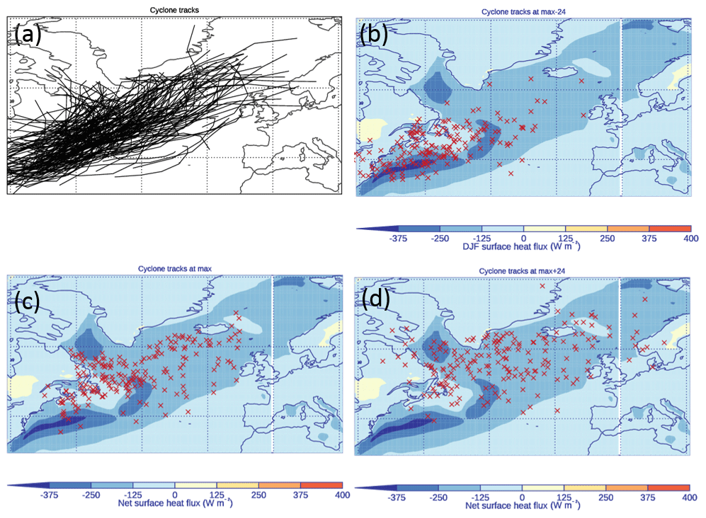
Figure 1(a) Tracks of the 200 most intense DJF North Atlantic storms between December 1989 and February 2009 (black). Position of the cyclones (b) 24 h before maximum intensity (max − 24), (c) at maximum intensity (max) and (d) 24 h after maximum intensity (max + 24; red crosses). Overlaid on the DJF North Atlantic 1989–2015 net surface heat flux climatology, QN (W m−2).
2.4 Cyclone-relative composites
The fields, described in Sect. 2.1, are extracted from ERA-Interim at each of the 6 hourly locations of the cyclone within a 30∘ radius surrounding the cyclone centre. Cyclone-relative composites are produced by averaging over all cyclones. Following Catto et al. (2010), before compositing, the fields are rotated according to the direction of travel of each cyclone such that the direction of travel in the composite becomes the same for all cyclones. Since the cyclones have quite different propagation directions, performing the rotation ensures that mesoscale features such as warm and cold fronts are approximately aligned and are not smoothed out by the compositing. As this method assumes that the cyclones all intensify and decay at the same rate, only the 200 most intense cyclones are included in the composite. The 850 hPa relative vorticity mean and standard deviation of the of these cyclone are shown in (Dacre et al., 2012; their Fig. 2c). Limiting the number of cyclones produces a more homogeneous group in terms of their evolution but will bias the mean fields towards being typical of the most intense cyclones. Data are only included in the composite where grid points lie over the ocean surface.
2.5 Cyclone and environmental flow partition
To understand the part played by cyclones in the development of the cold anomaly during the winter of 2013–2014 the net surface heat flux is partitioned into environmental and cyclone components. To partition QN into a part due to environmental flow and a part associated with cyclones we combine the cyclone tracks for that season with a masking method. A cyclone mask is calculated for each time step where the regions influenced by a cyclone are given a value of 1 (i.e. they are inside the cyclone mask), and regions that are not influenced are given a value of zero (i.e. they are outside the cyclone mask; Hawcroft et al., 2012; Sinclair and Dacre, 2019). The heat flux associated with cyclones is asymmetric around the cyclone. Large negative flux is found close to the cyclone centre and extending along the trailing cold front, which lies to the west of the cyclone centre. To account for this, a cyclone mask at a given time, t, is created by identifying the position of a cyclone and also its position during the previous 30 h representing the cyclone's cold wake. A mask is created which extends 14∘ in a radial circle from each track point, creating an elongated oval shape which encompasses both the cyclone centre and the cold wake (Fig. 2). This is equivalent to taking a swath with circles around all cyclone positions in the previous 30 h. The QN anomaly when cyclones are not present is associated with the environmental flow. The QN anomaly within the cyclone masks is associated with cyclones embedded within the environmental flow.
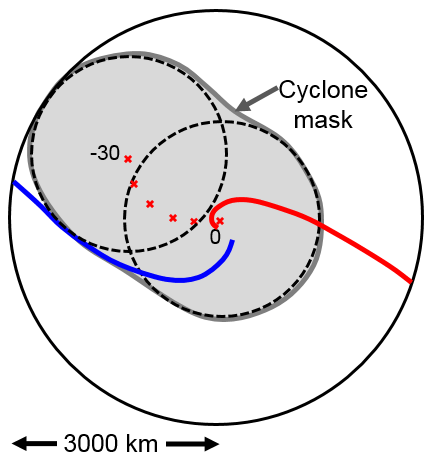
Figure 2Schematic of cyclone-masking method. Red and blue lines show the approximate position of the cyclone warm and cold front respectively. Red crosses show the position of a given cyclone at time (t) and at 6-hourly intervals up until 30 h previously (−30). The outer circle shows the 30∘ radius circle used to produce the composites in Figs. 5 to 8. The smaller dashed circles show example locations of a 14∘ radius circle centred on the cyclone position at t=0 and t=30. The grey shading shows the extent of the cyclone mask, encompassing the cyclone's centre and cold wake.
2.6 Sea surface temperature tendency
In order to calculate the SST tendency (ΔSST) we must take into account the MLD through which the heating or cooling due to the surface fluxes is mixed (h). Mixing in the ocean is assumed to occur between the surface and the MLD obtained from ORAS5. Assuming a well-mixed layer, the SST tendency due to QN and MLD (ΔSST) is given by
where ρ is the density of sea water, 1024 kg m−3, and cp is the specific heat capacity of sea water, 4000 J kg−1 K−1.
The SST tendency anomaly due to air–sea interactions (ASIs), ΔSST, for the 2013–2014 season is determined by subtracting the climatological SST tendency from the 2013–2014 SST tendency and is given by
where the overbar represents the 1989–2015 climatological value. The SST tendency anomaly can be separated into the anomaly associated with (i) anomalous QN (term 1 in Eq. 2), (ii) anomalous MLD (term 2 in Eq. 2) and (iii) anomalous entrainment through the base of the mixed layer, QENT (term 3 in Eq. 2). Since we have no measurements of the entrainment flux anomaly across the ocean boundary layer, it is estimated to be 20 % of the surface QN anomaly (Stull, 1988). This estimate for the entrainment flux neglects contributions made by wind-driven turbulence.
3.1 North Atlantic heat flux and SST tendency climatologies
Figure 3 shows the average heat flux for the period DJF 1989–2015 over the North Atlantic. The net surface solar radiation is positive, with a meridional gradient of 50 W m−2 1000 km−1, (Fig. 3a) and the net thermal radiation (Fig. 3b) is negative, with a magnitude between −50 and −100 W m−2. The sensible heat flux (Fig. 3c) is generally positive over land and negative over the ocean, with negative flux between −50 and −150 W m−2 in the Gulf Stream and Davis Strait regions, caused by the advection of cold air from the land over relatively warm oceans in DJF. The latent heat flux (Fig. 3d) is generally negative, with a band of enhanced negative flux extending in a north-eastwards direction from the East Coast of the US towards Iceland, with the values >200 W m−2 found in the west of the North Atlantic. The net heat flux, QN (Fig. 3e), is negative over the majority of the domain. A combination of QH and QE results in maximum negative heat flux >300 W m−2 in the Gulf Stream region. The largest QN values are co-located with the position of the North Atlantic storm track (Fig. 3f), which also exhibits a pronounced south-west–north-east tilt similar to the storm track in Fig. 1a.
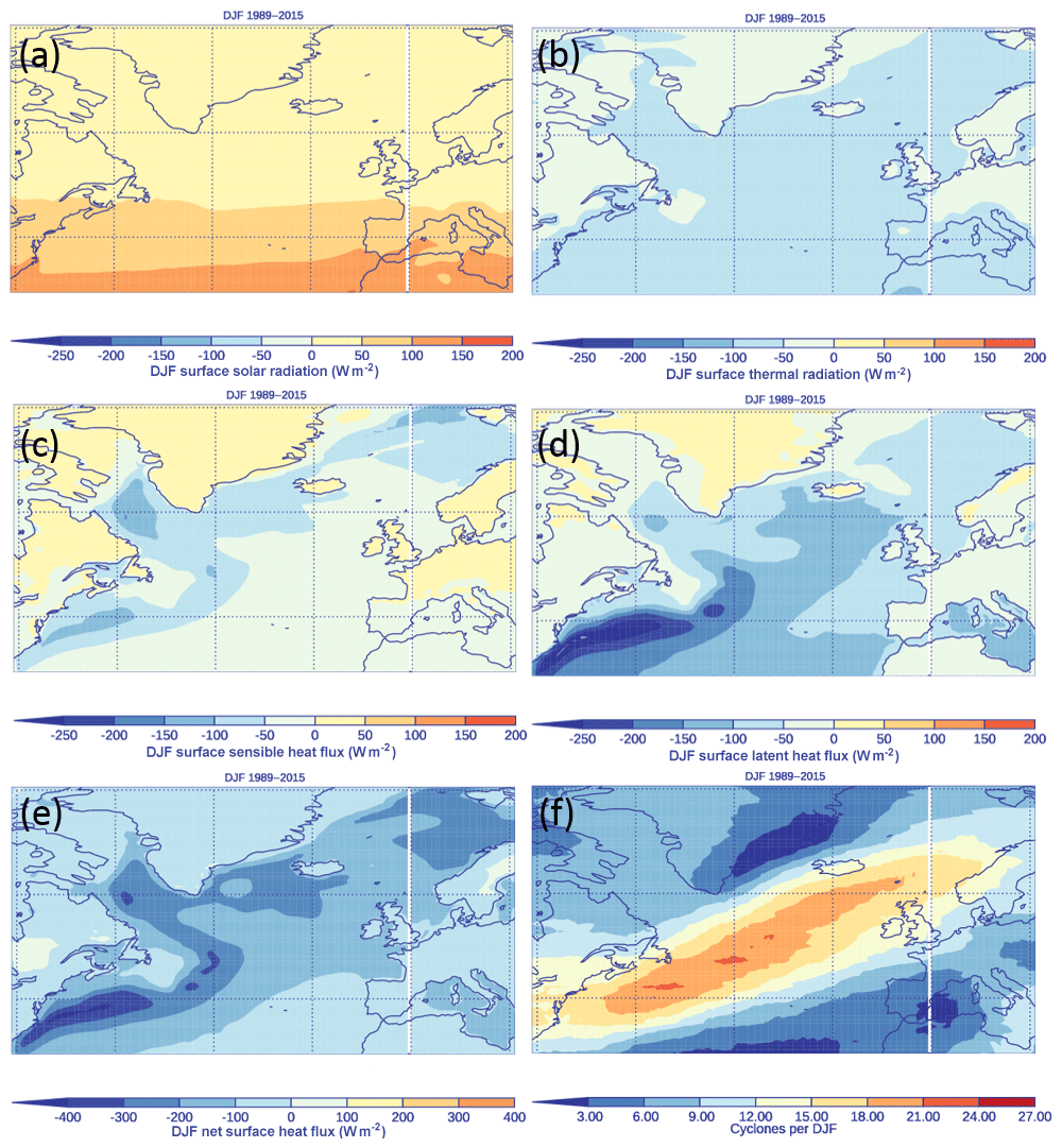
Figure 3North Atlantic 1989–2015 heat flux climatologies (W m−2). (a) Surface solar radiation QSW, (b) surface thermal radiation QLW, (c) surface sensible heat flux QH, (d) surface latent heat flux QE and (e) net surface heat flux QN. Note change in scale in (e). Positive flux is into the surface, and negative flux is into the atmosphere. (f) 1989–2015 climatological number of cyclones per DJF season within 12∘ of grid point.
Figure 4a and b show the climatological SST and the average SST change over DJF (ΔSSTTOT) for the period 1989–2015. During DJF the North Atlantic cools by an average of 2 K (Fig. 4b). The cooling is greatest where the SST gradient is largest in the Gulf Stream region (dotted box in Fig. 4a), with cooling of over 6 K over the winter. Unlike the climatological QN shown in Fig. 3e the region of highest ΔSSTTOT does not extend over the North Atlantic towards Iceland but remains close to the East Coast of the US.
In order to calculate the SST tendency due to QN we must take into account the MLD through which heating or cooling at the surface is mixed using Eq. (1). Figure 4c shows the climatological MLD. The MLD ranges from a few tens of metres close to Newfoundland to over 1000 m in the Labrador and Norwegian seas, where deep convection occurs. On average the MLD deepens by 50 % between December and February outside the deep convection regions (not shown). Taking the MLD into account restricts the largest ΔSST to the western North Atlantic region (Fig. 4d). The difference between ΔSSTTOT and ΔSST is shown in Fig. 4e. Differences >6 K are found close to the coast, where the western boundary currents transport warm waters north, resulting in reduced cooling over the DJF period than would be expected due to QN alone.
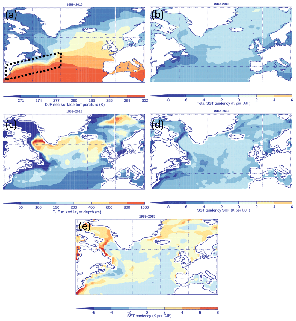
Figure 4North Atlantic DJF 1989–2015 (a) sea surface temperature (SST; K), black dotted box outlines region of the Gulf Stream, (b) ΔSSTTOT (K per DJF), (c) mixed layer depth (m), (d) ΔSST (K per DJF), and (e) difference between ΔSSTTOT and ΔSST.
3.2 Cyclone-relative heat flux composites
The north–south SST gradient in Fig. 4a is important for creating negative heat flux when cold dry air, from higher latitudes, is advected over relatively warm ocean surfaces. The largest heat flux occurs when large differences in temperature or moisture between the surface and overlying atmosphere are co-located with enhanced wind speeds. Given the spatial distribution of SSTs, atmospheric temperatures and moisture content, this is likely to occur when there are anomalously strong meridional winds such as those found ahead of and behind extratropical cyclones. Thus, whilst the maximum climatological SST gradient controls where locally high surface flux occurs, the presence of extratropical cyclones is likely to control when the largest heat flux occurs and its magnitude (Rudeva and Gulev, 2011; Ogawa and Spengler, 2019). In addition, the similarities between the spatial pattern of climatological QN (Fig. 3e) and cyclone numbers per season (Fig. 3f) suggest that cyclones play a role in generating QN. In this section we investigate QN in a cyclone-relative frame of reference using the methodology described in Sect. 2.3 and 2.4.
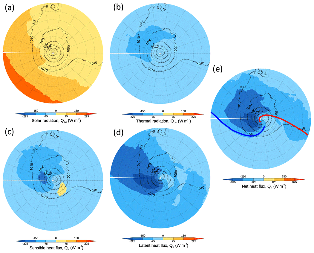
Figure 5Composite cyclone-centred heat fluxes (W m−2) for cyclones at maximum intensity. (a) Surface solar radiation QSW, (b) surface thermal radiation QLW, (c) surface sensible heat flux QH, (d) surface latent heat flux QE and (e) net surface heat flux QN overlaid with mslp. Note the change in colour scale in (e). Positive fluxes are into the surface, and negative fluxes are into the atmosphere. The radius of the circles is 3000 km, and the cyclones travel from left to right. The blue and red lines in (e) represent the approximate positions of the cold and warm fronts at max intensity.
Figure 5 shows composite cyclone-centred heat flux for the 200 most intense cyclones occurring between 1989 and 2009. The cyclones are at maximum intensity (maximum 850 hPa relative vorticity) when they are located at the centre of the domain and were rotated so that they all travel from left to right. QSW (Fig. 5a) contribution to QN is positive, and, like the Earth-relative perspective (Fig. 3a), there is a weak gradient. However, because the cyclones typically travel in a north-eastwards direction and they have been rotated, this gradient is also rotated. QLW (Fig. 5b) is negative everywhere and small, similar to the Earth-relative perspective. QLW is slightly enhanced in the region behind the cold front, potentially due to a reduction of cloud, which reduces the downwelling radiation. QH (Fig. 5c) shows a dipole structure at this stage in the cyclones' evolution, with negative flux behind the cyclone centre and positive flux in the cyclones' warm sector. QE (Fig. 5d) is negative everywhere, has its minimum in an extended region behind the cyclone and is reduced ahead of the cyclone. QN (Fig. 5e) is therefore negative surrounding the cyclone centre, with a minimum behind the cyclone. Negative flux >200 W m−2 occurs within 1000 km of the cyclone centre but extends almost 2000 km behind the cyclone due to a combination of QH and QE occurring behind the cold front.
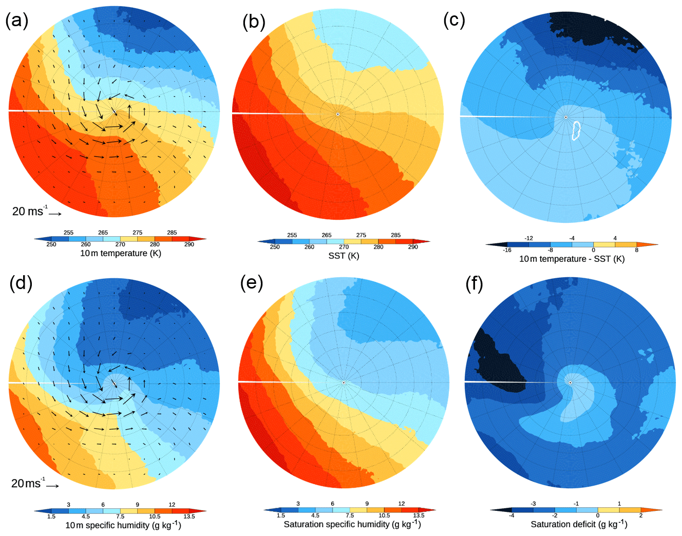
Figure 6Cyclone-centred fields at maximum intensity. (a) 10 m air temperature (K), (b) SST (K), (c) 10 m temperature − SST (white contour is −0.4 K; K), (d) 10 m specific humidity (g kg−1), (e) saturation humidity of SST (g kg−1), and (f) 10 m specific humidity − saturation humidity of SST (g kg−1). Panels (a) and (d) overlaid with 925 hPa winds.
In order to illustrate the processes leading to negative QH behind the cyclone cold front and positive QH in the warm sector it is necessary to examine the temperature characteristics of the different air masses in these regions. Figure 6a shows the composite 10 m air temperature overlaid with 925 hPa winds, and Fig. 6b shows the SST. The 10 m air temperature exhibits a wave-like structure, whilst the SST gradient is more linear. This results in a large negative near surface temperature difference (SST > 10 m temperature) behind the cold front. Cyclonic winds advect relatively cold air over a warm ocean surface behind the cyclone, resulting in negative QH. Ahead of the cyclone cyclonic winds advect warm air over the ocean surface; 6 h before maximum intensity, SST < 10 m air temperature ahead of the cyclone (not shown), but at maximum intensity the difference is close to zero (white contour in Fig. 6c shows −0.4 K). Since QH is a 6 h average, this results in the positive QH observed in Fig. 5c. Figure 6d and e show the 10 m specific humidity and the saturation specific humidity at the SST respectively. The 10 m specific humidity also has a pronounced wave structure, with drier air behind the cold front and moister air in the warm sector. Behind the cold front the saturation deficit is >4 g kg−1 (Fig. 6f), causing evaporation of moisture from the surface and large negative QE observed in Fig. 5d. Ahead of the cyclone the moisture deficit is <1 g kg−1, significantly reducing the magnitude of QE.
Figure 7a–c show composite QN centred on cyclones at different stages in their evolution. As the cyclones start to intensify negative QN behind the cold front strengthens (Fig. 7b). During the mature stages of the cyclone evolution (Fig. 7c) QN begins to decrease and to wrap cyclonically around the cyclone centre. This is due to the fact that the cold front typically rotates cyclonically towards the warm front as the cyclone reaches maturity. These results are consistent with the findings of Rudeva and Gulev (2011), who found that turbulent heat flux increases with cyclone intensity.
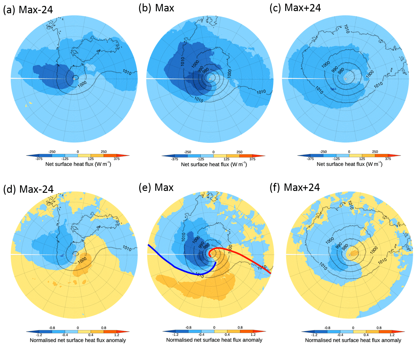
Figure 7Evolution of cyclone-centred (a–c) net surface heat flux QN (filled contours, W m−2), (d–f) normalized net heat flux anomaly (filled contours) and mslp (black contours; hPa). Cyclones reach the centre of the domain (a, d) 24 h before maximum intensity, (b, e) at maximum intensity and (c, f) 24 h after maximum intensity. In (d)–(f) negative normalized heat flux anomalies indicate anomalously large heat flux into the atmosphere, and positive anomalies indicate anomalously small heat flux into the atmosphere, compared to climatology. The blue and red lines in (e) represent the approximate positions of the cold and warm fronts at max intensity.
Interestingly, throughout the cyclone life cycle there is a secondary minimum in QN occurring approximately 2000 km ahead of the cyclone location. This secondary minimum does not change magnitude, so it is unlikely to be affected by the cyclones at the centre of the composite. It is possible that this second minimum is due the presence of a downstream cyclone, indicated by the composite mean sea-level pressure (mslp) contours, which extends towards the upper-right quadrant of the domain.
Since many of the 200 cyclones contributing to the composite QN (Fig. 5e) are generated over the Gulf Stream region it is possible that large negative QN occurring behind of the cyclone centre could be an artefact of their preferential cyclogenesis over a region of climatologically large negative QN (Fig. 3e). To determine how QN compares to the background values, we normalize QN anomalies by subtracting the climatological field at the position of each cyclone and dividing by the standard deviation of the climatology at the same location. Figure 7d–f show normalized QN anomalies at different stages of the cyclone evolution. Negative anomalies indicate anomalously large heat flux into the atmosphere, with a value of −1 being 1 SD (standard deviation) larger than the climatological mean. Positive anomalies indicate anomalously small heat flux into the atmosphere, with a value of +1 being 1 SD smaller than the climatological mean. At all stages of the cyclone evolution negative QN behind the cyclone centre is more than 0.5 SD greater than the mean for strong cyclones and is more than 1 SD greater than the mean at maximum intensity (Fig. 7e). Ahead of the cyclone QN is 0.4–0.8 SD greater than the mean at maximum intensity (Fig. 7e) due to warm air advection in the warm sector of the cyclone. Note that towards the edges of the domain many of the grid points are over land, so they have been excluded; therefore the sample size contributing to the composites is small, resulting in a noisy field.

Figure 8Evolution of cyclone-centred (a–c) ΔSST (filled contours; K 12 h−1), (d–f) normalized ΔSST anomaly (filled contours) and mslp (black contours; hPa). Cyclones reach the centre of the domain (a, d) 24 h before maximum intensity, (b, e) at maximum intensity and (c, f) 24 h after maximum intensity. In (d)–(f) negative normalized ΔSST anomalies indicate anomalously large SST cooling due to QN, and positive anomalies indicate anomalously small SST cooling, compared to climatology.
3.3 Cyclone-relative SST tendency
Using Eq. (1) the evolution of the cyclone-relative SST tendencies due to QN can be estimated. Figure 8 shows ΔSST per day for cyclones at different stages in their evolution. The patterns of ΔSST are similar to the patterns of QN (Fig. 7a–c), showing that the surface flux is the dominant variable in the cooling and that variations in mixed layer depth are less important. As for QN, ΔSST increases as the cyclones reach maximum intensity, with maximum SST tendencies of 0.2 K d−1 occurring in the cold sector behind the cold front. The normalized ΔSST anomalies are calculated by subtracting the climatological ΔSSTTOT and dividing by the standard deviation of ΔSSTTOT (Fig. 8d–f). ΔSST is larger than the climatological mean behind the cold front. However in this case the intense cyclones only reduce ΔSST by up to 0.25 times the standard deviation.
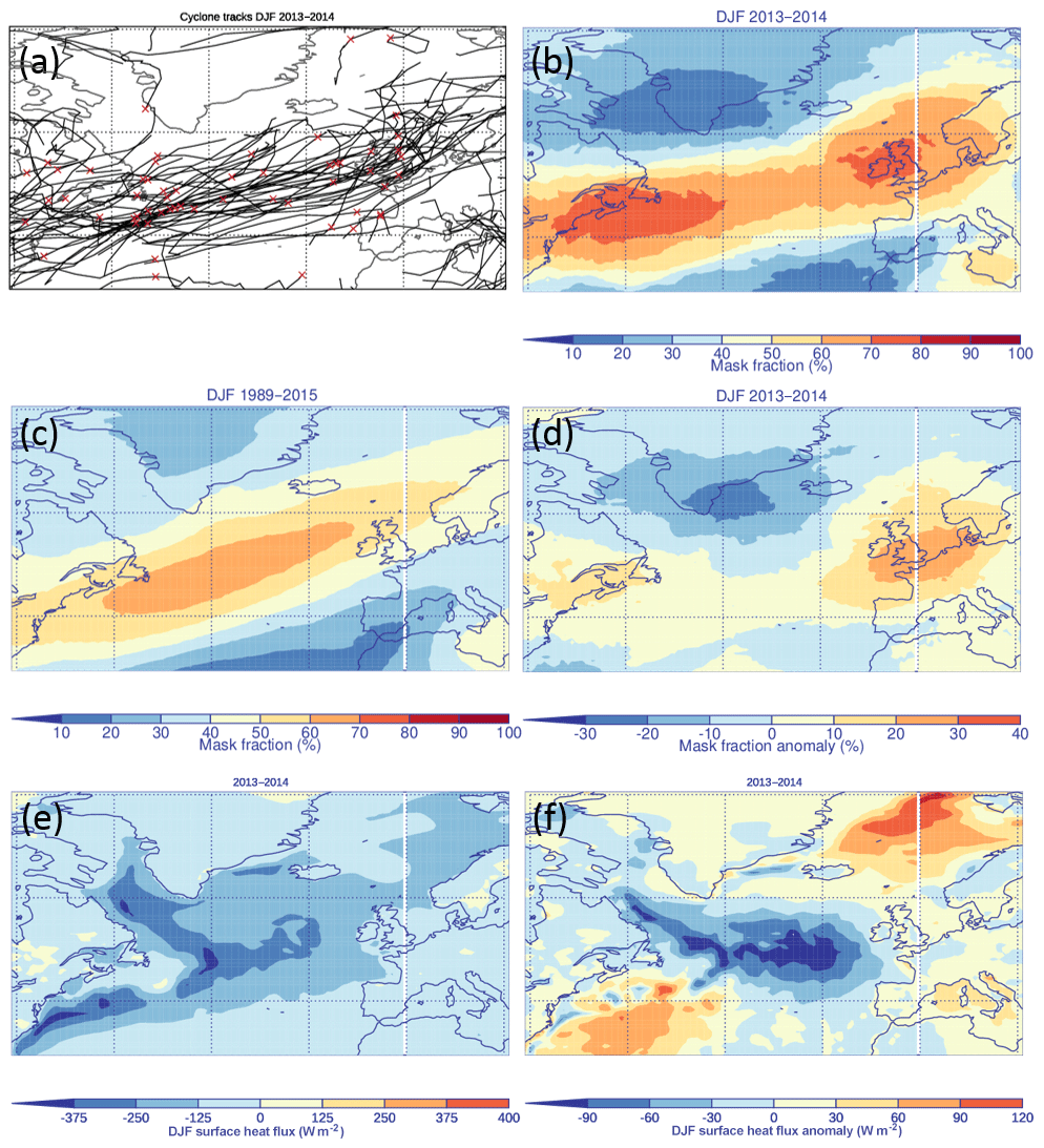
Figure 9(a) 2013–2014 cyclone tracks (black) with position of maximum intensity (red crosses), (b) 2013–2014 fraction of time within cyclone mask, (c) 1989–2015 mask fraction, (d) anomalous mask fraction, (e) 2013–2014 QN (W m−2) and (f) anomalous QN (W m−2).
ΔSST cooling associated with each individual extratropical cyclone is of the order of 0.1–0.2 K d−1 (Fig. 8a–c); therefore if many cyclones track over the same location we might expect to see a signature of the storm track in the seasonal QN and SST anomaly patterns. Figure 9a shows the tracks of cyclones in the North Atlantic region. Applying the cyclone-masking methodology described in Sect. 2.6 to the 2013–2014 winter cyclones, we see that the cyclones track in a south-west–north-east direction in a narrow band that extends from the East Coast of the US towards the UK (Fig. 9b). This season was unusually stormy in the UK, with cyclones passing over the UK every 3 d (Priestley et al., 2017). The effect of propagation speed is taken into account in the masking methodology, since multiple time steps for a single cyclone contribute to the seasonal mask fraction. We also apply the cyclone-masking methodology to winter cyclones between 1989 and 2015 (Fig. 9c) and find that, in comparison to the 1989–2015 average, in 2013–2014 the storm track was more active, with a higher number of cyclones, and also more zonal than usual (Fig. 9d). This was associated with an anomalously strong and zonally elongated upper-level westerly jet in 2013–2014 (Kendon and McCarthy, 2015). More cyclones travelled towards western Europe and Iceland than usual.
It was shown in Fig. 7 that intensifying cyclones create negative QN behind the cold front, where cold dry air is advected over a warm ocean surface. Therefore we hypothesize that an anomalously strong and zonal storm track will result in an anomalously strong and zonally orientated seasonal QN anomaly. The 2013–2014 DJF season QN is shown in Fig. 9e, and the 2013–2014 QN anomaly is shown in Fig. 9f. The seasonal QN anomaly has a tripole pattern, with stronger negative QN in the mid-North Atlantic and weaker negative QN over the Gulf Stream and in the Norwegian and Greenland seas. In the mid-Atlantic this is consistent with the shift in the storm track, with cyclones travelling more zonally from the US towards western Europe rather than north-eastwards towards Iceland.
Figure 10a and b show UK Met Office synoptic analysis charts at 00:00 UTC on 24 and 20 December 2013 respectively. At both times there is a low-pressure centre situated to the west of Scotland and long trailing cold fronts extending across the North Atlantic. Figure 10c and d show QN at the corresponding times, and Fig. 10e and f show the cyclone masks. The red lines show the full track of the cyclones, and the elongated oval masks the location of the cyclones at the analysis time and 30 h earlier. The mask captures QN surrounding the cyclone centres and the cyclone's cold wake. Sensitivity tests have been performed using a radial circle ranging from 12 to 16∘ and masks extending 24 to 36 h prior to the analysis time.
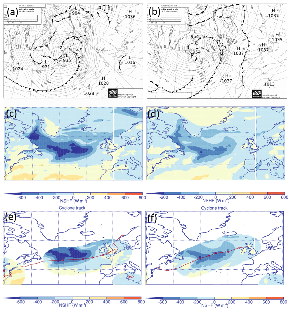
Figure 10(a, b) UK Met Office synoptic analysis charts, (c, d) QN (W m−2), and (e, f) cyclone mask overlaid with tracks for (a, c, e) 00:00 UTC 24 December 2013 and (b, d, f) 00:00 UTC 20 December 2013. Red crosses show the position of cyclones at the analysis time and 30 h previously.
4.1 2013–2014 SST anomalies
Figure 11a shows the 2013–2014 DJF SST tendency anomaly (ΔSST′) that is associated with anomalous QN. As expected ΔSST′ due to anomalous QN closely resembles the QN anomaly (shown in Fig. 9f), with anomalous cooling in the mid-North Atlantic, where the flux anomaly is negative and anomalous warming (less cooling than climatology) in the Gulf Stream and Norwegian Sea regions. Small differences are due to spatial inhomogeneity in the North Atlantic climatological MLD. Figure 11b shows the 2013–2014 DJF ΔSST′ that is associated with anomalous MLD. The 2013–2014 MLD is shallower than the climatological average over much of the domain, particularly near the Gulf Stream region, and deeper than climatology in the mid-Atlantic region. In the mid-North Atlantic the enhanced negative QN results in negative buoyancy and thus mixing, deepening the MLD. Therefore, the surface flux decreases the temperature over a deeper layer of the ocean than usual, which reduces the direct SST cooling due to QN. At the same time, the increased MLD mixes colder water from below into the mixed layer, which cools the surface indirectly. Figure 11c shows the sum of the ΔSST′ due to anomalous QN, anomalous MLD and anomalous entrainment (ΔSST). It shows the same tripole pattern as the ΔSSTTOT anomaly (Fig. 11d), which has an average SST cooling anomaly of −1.0 K in the mid-North Atlantic region (black box in Fig. 11d). In the mid-North Atlantic region, the ΔSST accounts for 68 % of the total anomalous SST cooling in the mid-North Atlantic. The largest discrepancies occur along the eastern coast of North America, suggesting that ocean dynamics are responsible for transporting warmer and colder water into these regions via the western boundary currents. For example, off the coast of Nova Scotia the SSTs are very cold, since the Labrador current flows south from the Arctic Ocean. Advection of relatively warm air over these cold SSTs in a region where the mixed layer depth is shallow results in a positive SST tendency anomaly.
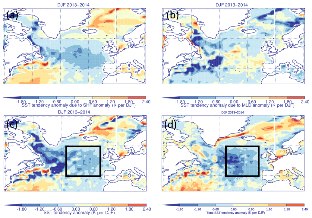
Figure 11Anomalous ΔSST due to 2013–2014 (a) QN (SHF) anomaly, (b) MLD anomaly and (c) ΔSSTASI anomaly. (d) ΔSSTTOT anomaly.
4.2 2013–2014 cyclone and environmental flow SST anomalies
In this section we partition the QN anomaly into a part associated with the environmental flow (i.e. outside the cyclone masks described in Sect. 2.6) and a part associated with the presence of cyclones (inside the cyclone masks described in Sect. 2.6). Figure 12a shows the contribution to the DJF QN anomaly due to both cyclones and the environmental flow, and Fig. 12b shows the contribution that is due to the environmental flow only. Both Fig. 12a and b show a tripole pattern, with anomalously negative heat flux between 40 and 60∘ N and anomalously positive heat flux over the Gulf Stream and Norwegian seas. This suggests that the overall pattern is controlled by the environmental flow. The anomalously positive heat flux in the Norwegian Sea and Gulf Stream region may be due to a reduced number of cold-air outbreaks (Papritz and Spengler, 2017; Papritz and Grams, 2018; Parfitt et al., 2016). In the mid-North Atlantic the negative QN anomaly is enhanced, compared to contribution made by the environment (doubled from 32 % to 68 % of the total seasonal QN anomaly), when cyclones are present. In the Norwegian Sea and Mediterranean Sea the positive QN anomaly due to the environmental flow is suppressed by the presence of cyclones. Thus cyclones embedded within the environmental flow pattern tend to increase the negative surface heat flux, consistent with the cyclone-relative results in Sect. 3.2. Varying the size of the cyclone mask radius from 12 to 16∘ results in a contribution to the total QN anomaly when cyclones are present in the mid-North Atlantic that ranges from 62 % to 72 %, and varying the length of the cyclone mask from 24 to 36 h results in a cyclone contribution from 62 % to 71 %. This suggests that the conclusion that cyclones enhance the QN anomaly does not depend strongly on the choices used to define the cyclone mask.
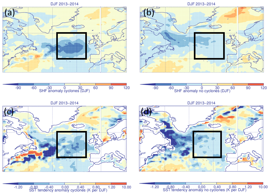
Figure 122013–2014 anomalous QN associated with (a) both cyclones and the environmental flow and (b) the environmental flow. 2013–2014 anomalous ΔSST due to anomalous QN, MLD and entrainment associated with (c) both cyclones and the environmental flow and (d) the environmental flow.
Figure 12c shows the contribution to the 2013–2014 ΔSST due to both cyclones and the environmental flow, and Fig. 12d shows the contribution that is due to the environmental flow only. As for the QN anomaly, both show a tripole pattern, suggesting that the environmental flow controls the anomalously large cooling in the mid-North Atlantic and the anomalously small cooling in the Norwegian Sea and Gulf Stream regions. In the mid-North Atlantic region, the negative ΔSST is also enhanced (from 28 % to 41 % of the total seasonal ΔSST′) when cyclones are present. This is less than their added contribution to the 2013–2014 QN anomaly because the enhanced negative QN cools a deeper layer of the ocean than usual, which reduces the direct SST cooling.
In this paper we investigate both the SST cooling associated with individual cyclones and the SST cooling associated with the passage of multiple cyclones over the same location in the 2013–2014 season to determine how significant cyclones were in contributing to the anomalously large cooling that occurred during the 2013–2014 winter. We find that enhanced air–sea exchange of heat and moisture in the cold sector behind the cold front of an extratropical cyclone can lead to cooling of up to 0.2 K d−1 for the strongest cyclones. This cooling is relatively small compared to the variability in SST tendency in the North Atlantic; thus the cold wake associated with the passage of an individual extratropical cyclone is difficult to observe in the instantaneous SST field.
During the 2013–2014 DJF season there was a zonal band of anomalously large negative heat fluxes extending from the East Coast of the US towards Europe. The mixed layer depth was also anomalously deep in the mid-North Atlantic due to enhanced mixing and entrainment of water into the mixed layer from below. The combination of these air–sea interactions accounts for 68 % of the total ΔSST anomaly. Thus air–sea interactions were very important in determining the anomalous SST cooling between December 2013 and February 2014.
In 2013–2014 the environmental flow pattern was anomalously zonal compared to climatology over the North Atlantic. This resulted in anomalously negative heat flux between 40 and 60∘ N and anomalously positive heat flux over the Norwegian and Gulf Stream regions. When cyclones were present, heat flux from the ocean to the atmosphere was doubled in the mid-North Atlantic region. The enhancement of the negative heat flux caused a direct cooling of the ocean but also led to increased entrainment and thus a deeper mixed layer. This deepening reduces the overall effect of the cooling, as the heat loss acts on a greater volume of water than normal. Consequently, while the SST tendency anomaly in the mid-North Atlantic was enhanced by the presence of cyclones, it was by a smaller amount than might be expected due to a doubling of the heat flux. We conclude that both the environmental flow and extratropical cyclones embedded within this flow played important roles in determining the extreme 2013–2014 winter season SST cooling.
The ERA-Interim data were obtained freely from https://www.ecmwf.int/en/forecasts/datasets/reanalysis-datasets/era-interim (last access: February 2020; Dee et al., 2011). The ORAS5 data were obtained freely from the Integrated Climate Data Center at the University of Hamburg: http://icdc.cen.uni-hamburg.de (last access: February 2020). Information on how to obtain the cyclone identification and tracking algorithm can be found from http://www.nerc-essc.ac.uk/~kih/TRACK/Track.html (last access: February 2020), and access can be obtained by emailing Kevin Hodges (k.i.hodges@reading.ac.uk).
HFD performed the data analysis for this publication. SAJ and ALMG contributed to the scientific interpretation of the analysis.
The authors declare that they have no conflict of interest.
We thank Kevin Hodges for providing their ETC tracking code. Simon A. Josey receives funding from the UK Natural Environment Research Council, including the ACSIS and EMERGENCE programmes.
Simon A. Josey acknowledges funding from the UK Natural Environment Research Council under the North Atlantic Climate System Integrated Study program (reference number NE/N018044/1).
This paper was edited by Shira Raveh-Rubin and reviewed by three anonymous referees.
Alexander, M. A. and Scott, J. D.: Surface flux variability over the North Pacific and North Atlantic oceans, J. Climate, 10, 2963–2978, 1997. a
Buckley, M. W., Ponte, R. M., Forget, G., and Heimbach, P.: Determining the origins of advective heat transport convergence variability in the North Atlantic, J. Climate, 28, 3943–3956, 2015. a
Catto, J. L., Shaffrey, L. C., and Hodges, K. I.: Can climate models capture the structure of extratropical cyclones?, J. Climate, 23, 1621–1635, 2010. a
Courtois, P., Hu, X., Pennelly, C., Spence, P., and Myers, P. G.: Mixed layer depth calculation in deep convection regions in ocean numerical models, Ocean Model., 120, 60–78, 2017. a
Crawford, G. and Large, W.: A numerical investigation of resonant inertial response of the ocean to wind forcing, J. Phys. Oceanogr., 26, 873–891, 1996. a
Dacre, H. F., Hawcroft, M. K., Stringer, M. A., and Hodges, K. I.: An extratropical cyclone atlas: A tool for illustrating cyclone structure and evolution characteristics, B. Am. Meteorol. Soc., 93, 1497–1502, 2012. a, b
Dacre, H. F., Martinez-Alvarado, O., and Mbengue, C. O.: Linking atmospheric rivers and warm conveyor belt airflows, J. Hydrometeorol., 20, 1183–1196,, 2019. a
Dee, D. P., Uppala, S., Simmons, A., Berrisford, P., Poli, P., Kobayashi, S., Andrae, U., Balmaseda, M., Balsamo, G., Bauer, D. P., and Bechtold, P.: The ERA-Interim reanalysis: Configuration and performance of the data assimilation system, Q. J. Roy. Meteorol. Soc., 137, 553–597, 2011. a
Fisher, E. L.: Hurricanes and the sea-surface temperature field, J. Meteorol., 15, 328–333, 1958. a
Grist, J. P., Josey, S. A., Jacobs, Z. L., Marsh, R., Sinha, B., and Van Sebille, E.: Extreme air–sea interaction over the North Atlantic subpolar gyre during the winter of 2013–2014 and its sub-surface legacy, Clim. Dynam., 46, 4027–4045, 2016. a
Hawcroft, M., Shaffrey, L., Hodges, K., and Dacre, H.: How much Northern Hemisphere precipitation is associated with extratropical cyclones?, Geophys. Res. Lett., 39, L24809, https://doi.org/10.1029/2012GL053866, 2012. a
Hodges, K.: Feature tracking on the unit sphere, Mon. Weather Rev., 123, 3458–3465, 1995. a
Kawai, Y. and Wada, A.: Detection of cyclone-induced rapid increases in chlorophyll-a with sea surface cooling in the northwestern Pacific Ocean from a MODIS/SeaWiFS merged satellite chlorophyll product, Int. J. Remote Sens., 32, 9455–9471, 2011. a
Kendon, M. and McCarthy, M.: The UK's wet and stormy winter of 2013/2014, Weather, 70, 40–47, 2015. a
Kleinschmidt, E.: Principles of the theory of tropical cyclones, Arch. Meteor. Geophys. Bioklimatol., 4, 53–72, 1951. a
Kobashi, F., Doi, H., and Iwasaka, N.: Sea surface cooling induced by extratropical cyclones in the subtropical North Pacific: Mechanism and interannual variability, J. Geophys. Res.-Oceans, 124, 2179–2195, 2019. a, b
Nelson, J., He, R., Warner, J. C., and Bane, J.: Air–sea interactions during strong winter extratropical storms, Ocean Dynam., 64, 1233–1246, 2014. a, b
Ogawa, F. and Spengler, T.: Prevailing Surface Wind Direction during Air-Sea Heat Exchange, J. Climate, 32, 5601–5617, 2019. a, b
Papritz, L. and Grams, C. M.: Linking low-frequency large-scale circulation patterns to cold air outbreak formation in the northeastern North Atlantic, Geophys. Res. Lett., 45, 2542–2553, 2018. a
Papritz, L. and Spengler, T.: Analysis of the slope of isentropic surfaces and its tendencies over the North Atlantic, Q. J. Roy. Meteorol. Soc, 141, 3226–3238, 2015. a
Papritz, L. and Spengler, T.: A Lagrangian climatology of wintertime cold air outbreaks in the Irminger and Nordic Seas and their role in shaping air–sea heat fluxes, J. Climate, 30, 2717–2737, 2017. a
Papritz, L., Pfahl, S., Sodemann, H., and Wernli, H.: A climatology of cold air outbreaks and their impact on air–sea heat fluxes in the high-latitude South Pacific, J. Climate, 28, 342–364, 2015. a
Parfitt, R., Czaja, A., Minobe, S., and Kuwano-Yoshida, A.: The atmospheric frontal response to SST perturbations in the Gulf Stream region, Geophys. Res. Lett., 43, 2299–2306, 2016. a, b
Parfitt, R., Czaja, A., and Kwon, Y.-O.: The impact of SST resolution change in the ERA-Interim reanalysis on wintertime Gulf Stream frontal air-sea interaction, Geophys. Res. Lett., 44, 3246–3254, 2017. a
Persson, G., Ola, P., Hare, J., Fairall, C., and Otto, W.: Air–sea interaction processes in warm and cold sectors of extratropical cyclonic storms observed during FASTEX, Q. J. Roy. Meteorol. Soc., 131, 877–912, 2005. a
Pettersen, S., Bradbury, D. L., and Pedersen, K.: The Norwegian cyclone models in relation to heat and cold sources, Geophysica Norvegica, 243–280, 1962. a
Priestley, M. D., Pinto, J. G., Dacre, H. F., and Shaffrey, L. C.: The role of cyclone clustering during the stormy winter of 2013/2014, Weather, 72, 187–192, 2017. a
Ren, X., Perrie, W., Long, Z., and Gyakum, J.: Atmosphere–ocean coupled dynamics of cyclones in the midlatitudes, Mon. Weather Rev., 132, 2432–2451, 2004. a, b
Rudeva, I. and Gulev, S. K.: Composite analysis of North Atlantic extratropical cyclones in NCEP–NCAR reanalysis data, Mon. Weather Rev., 139, 1419–1446, 2011. a, b, c, d
Schemm, S. and Sprenger, M.: Frontal-wave cyclogenesis in the North Atlantic – a climatological characterisation, Q. J. Roy. Meteorol. Soc., 141, 2989–3005, 2015. a
Shaman, J., Samelson, R., and Skyllingstad, E.: Air–sea fluxes over the Gulf Stream region: Atmospheric controls and trends, J. Climate, 23, 2651–2670, 2010. a
Sinclair, V. and Dacre, H.: Which Extratropical Cyclones Contribute Most to the Transport of Moisture in the Southern Hemisphere?, J. Geophys. Res.-Atmos., 124, 2525–2545, 2019. a
Stull, R. B.: An introduction to boundary layer meteorology, in: vol. 13, Springer, Dordrecht, 1988. a
Tanimoto, Y., Nakamura, H., Kagimoto, T., and Yamane, S.: An active role of extratropical sea surface temperature anomalies in determining anomalous turbulent heat flux, J. Geophys. Res.-Oceans, 108, 3304, https://doi.org/10.1029/2002JC001750, 2003. a
Toyoda, T., Fujii, Y., Kuragano, T., Kamachi, M., Ishikawa, Y., Masuda, S., Sato, K., Awaji, T., Hernandez, F., Ferry, N., and Guinehut, S.: Intercomparison and validation of the mixed layer depth fields of global ocean syntheses, Clim. Dynam., 49, 753–773, 2017. a
Vannière, B., Czaja, A., Dacre, H., and Woollings, T.: A “cold path” for the Gulf Stream–troposphere connection, J. Climate, 30, 1363–1379, 2017. a
Yao, Y., Perrie, W., Zhang, W., and Jiang, J.: Characteristics of atmosphere-ocean interactions along North Atlantic extratropical storm tracks, J. Geophys. Res.-Atmos., 113, D14124, https://doi.org/10.1029/2007JD008854, 2008. a
Zolina, O. and Gulev, S. K.: Synoptic variability of ocean–atmosphere turbulent fluxes associated with atmospheric cyclones, J. Climate, 16, 2717–2734, 2003. a
Zuo, H., Balmaseda, M., de Boisseson, E., Hirahara, S., Chrust, M., and De Rosnay, P.: A generic ensemble generation scheme for data assimilation and ocean analysis, European Centre for Medium-Range Weather Forecasts, ECMWF, available at: https://www.ecmwf.int/publications (last access: February 2020), 2017. a
Zuo, H., Balmaseda, M. A., Tietsche, S., Mogensen, K., and Mayer, M.: The ECMWF operational ensemble reanalysis–analysis system for ocean and sea ice: a description of the system and assessment, Ocean Sci., 15, 779–808, https://doi.org/10.5194/os-15-779-2019, 2019. a